
FLUENT’s Erosion Model to Investigate Erosion in a 90 degree Elbow Bend. Setup and Solution.
Following the steps of the tutorial provided by FLUENT, after the mesh was created (see details), the next thing to do is setting up all solver parameters:
- Model: The turbulence model suggested for this pipe is k-epsilon with standard wall function and default settings. Discrete Phase Model is set to iterate once ever 5 Continuous Phase iterations.
- Materials: The fluid element is water mixed with sand which forms some sort of slurry. Sand particles are of 2 microns in diameter.
- Boundary conditions: We have three boundaries, namely velocity inlet, outflow and wall. The velocity of the slurry is 10 m/s and a polynomial profile was used to define the Discrete Phase Reflection Coefficients.
- Solution methods and controls: A new monitor was set to follow the evolution of Static Pressure at the outlet. Solution was initialized with a Turbulent Dissipation Rate of 1×10⁵ m2/s3.
- Solve: According to the tutorial, the solution would converge in approximately 300 iterations. Calculations were run in only one processor, because when trying to go Parallel, having Discrete Phase On, some warnings would arise and solution for x-momentum diverged.
OMP: Warning #2: Cannot open message catalog "3082libguide40ui.dll":

OMP: System error #126: The specified module could not be found.

OMP: Info #3: Default messages will be used.
After 500 iterations we had a converged solution. In Figure 1 we can see the sand particle traces. The behavior we see is in concordance with investigations from authors such as Chen et al. [1] or Akilli et al. [2].
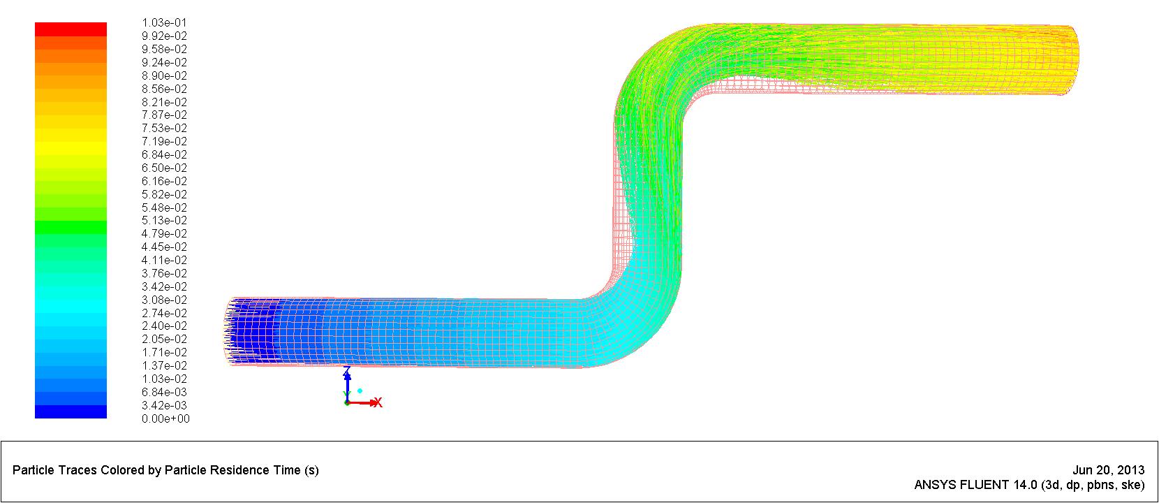
Figure 1. Particle traces.
Watching the particle traces we can guess where the eroded areas are to be located, which we can confirm with the contours of DPM erosion shown in Figure 2. We can clearly see that the maximum erosive location in the first elbow is not aligned with the incident axis of the pipe as a stochastic particle model would suggest. But according to Zhang et al. [3], the maximum erosive location moves downstream when slurry velocity increases; also, the impact force is higher when the slurry velocity is higher.
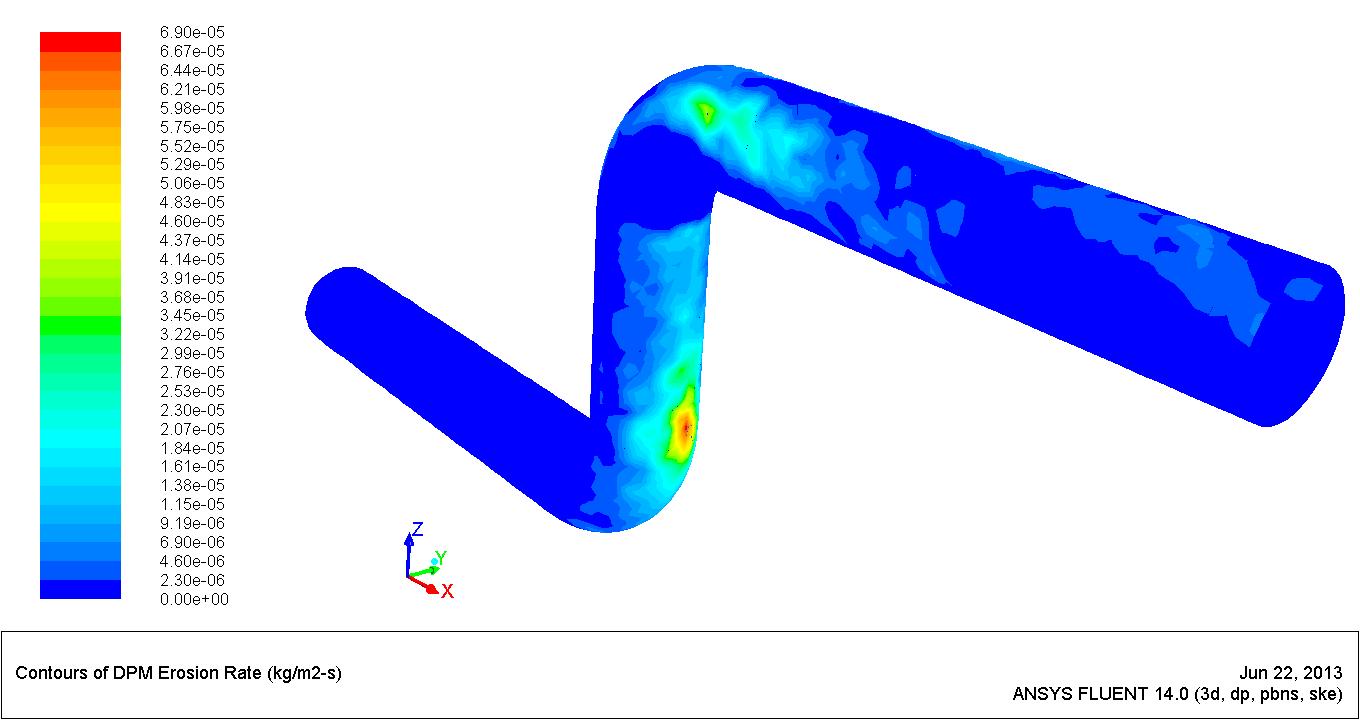
Figure 2. Contours of DPM erosion rate.
Maximum erosion rate is of 7.461 × 10⁻⁵ kg/m2s in the first elbow and of 5.877 × 10⁻⁵ kg/m2s in the second elbow, and if on a large radius elbow, we would see three or more erosion zones and some erosion free areas along the concave wall of the pipe, Njobuenwu and Fairweather [4].
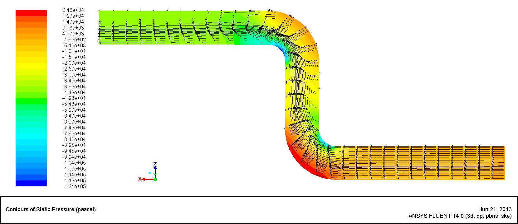
Figure 3. Contours of static pressure and vectors of velocity magnitude.
In addition to what is specified in the tutorial, in Figure 3 we have plotted the contours of static pressure alongside vectors of velocity magnitude which give a hint of where sand ropes might form and disperse.
References
[1] Chen, X., McLaury, B.S., y Shirazi, S.A. “Application and experimental validation of a computational fluid dynamics (CFD)-based erosion prediction model in elbows and plugged tees.” Computers & Fluids, 33(10), pages 1251 – 1272 (2004).
[2] Akilli, H., Levy, E., y Sahin, B. “Gas-solid flow behavior in a horizontal pipe after a 90º vertical-to-horizontal elbow.” Powder Technology, 116(1), pages 43 – 52 (2001).
[3] Zhang, H., Tan, Y., Yang, D., et al. “Numerical investigation of the location of maximum erosive wear damage in elbow: Effect of slurry velocity, bend orientation and angle of elbow.” Powder Technology, 217(0), pages 467 – 476 (2012).
[4] Njobuenwu, D.O. y Fairweather, M. “Modelling of pipe bend erosion by dilute particle suspensions.” Computers & Chemical Engineering, 42(0), pages 235 – 247 (2012).
What next
I am curious about how Dyson’s bladeless fans work, so I am planning to do a 2D axi-symmetric study on how air velocity flowing out of the ring affects different parameters.