
Lift and airfoils in 2D at subsonic speeds
In this post we will analyse some of the most widespread misconceptions regarding the lift of airfoils at subsonic speeds and try to give a more correct physical explanation of the phenomenon. This post is based mainly on what is exposed in the homonymous chapter of McLean’s work (2012). The explanations will be complemented with contributions from works that are a reference in aerodynamics, such as Anderson (2011) or White (2011), and with illustrations from CFD simulations that we have validated in 2D NACA 0012 airfoil validation.
Contents
Common misconceptions regarding lift
It is important to keep track of all assumptions that are used in the derivation of any equation because they tell you the limitations on the final result, and therefore prevent you from using an equation for a situation in which it is not valid.
John D. Anderson, Fundamentals of Aerodynamics.
Bernoulli’s equation
Bernoulli’s equation represents the relation between pressure and velocity in a inviscid, incompressible flow.
$$ p + \frac{1}{2}\rho V^2 = \text{constant} \qquad \text{along a streamline} $$
The equation was derived from the momentum equation, assuming an incompressible, inviscid flow with no body forces. Moreover, if the flow is irrotational, Bernoulli’s equation holds throughout the flow, not just the same streamline. Therefore, we need to verify the following assumptions in the vicinity of the airfoil:
Incompressible flow
The flow is usually considered incompressible when Mach < 0.3, as the differences in density are less than 5%, which can be considered negligible for practical purposes.
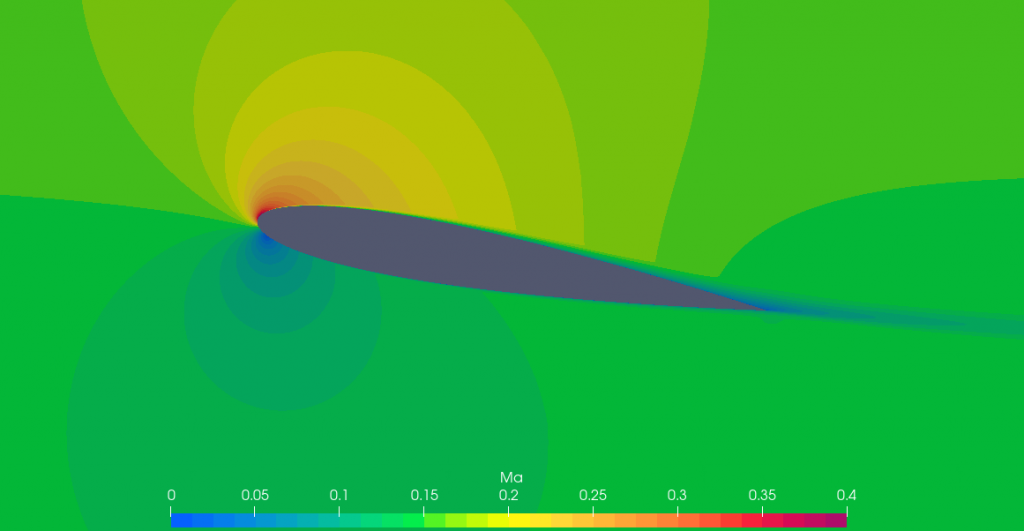
In the previous picture, even though the farfield Mach is just 0.15, near the leading edge around the region of lowest pressure, Mach number reaches values up to 0.4. It is certainly not a very large region, but it is the one that contributes the most to the lift generated by the airfoil (see the surface pressure chart here). As to how this affects density, we can see in the following picture.
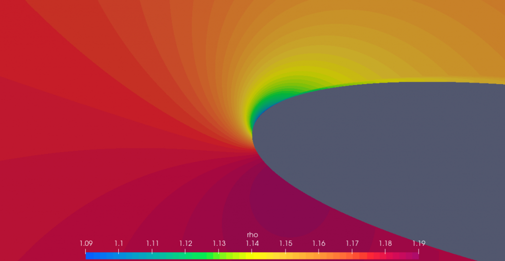
In our case, $\rho_\rm{ref}$ is 1.177 kg.m-3, thus, the lower range for still considering valid the no-compressibility assumption would be 1.118 kg.m-3. However, here we see that the density becomes lower than that, coinciding at the points where the speed is the highest.
In this case, the area outside the validity range of the assumption is very small, so the assumption is unlikely to induce much error.
Inviscid flow
Flows at high Reynolds numbers can be considered inviscid for most practical purposes. There’s though a small region close to the airfoil surface where the influence of friction, thermal conduction, and diffusion is important: the boundary layer. As the angle of attack is increased, the boundary layer will tend to separate, and a wake will form downstream.
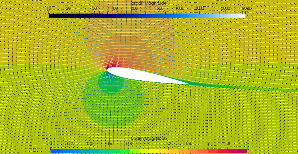
OpenFOAM has a field function that can determine the type of flow, flowType. We show the output of this field function in the following figure.
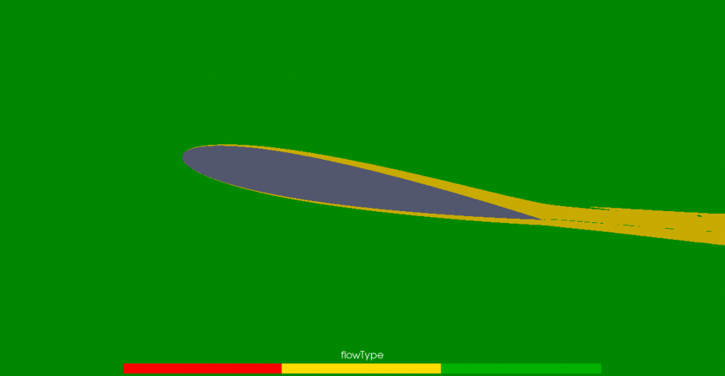
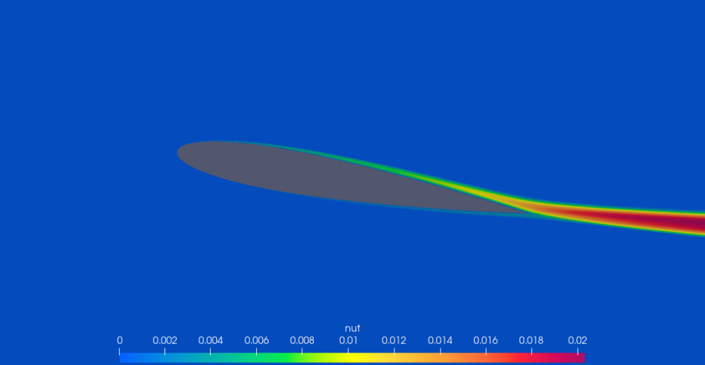
The yellow region is dominated by shear —viscous flow— while the green region is essentially inviscid flow. Not to mention that the region of viscous flow correlates quite well with eddy viscosity, shown below.
Body forces
Forces due to gravity, electric fields and magnetic fields are usually negligible. In the case we are most interested in, which is gravity, the difference in height is so small that the variation in potential energy is inconsequential.
Irrotational flow
We define a flow a flow as irrotational when the curl of the velocity —vorticity— is zero:
$$ \xi = \nabla \times \mathbf{V} = 0 $$
We used the vorticity field function in OpenFOAM to plot the regions where vorticity is non-zero.
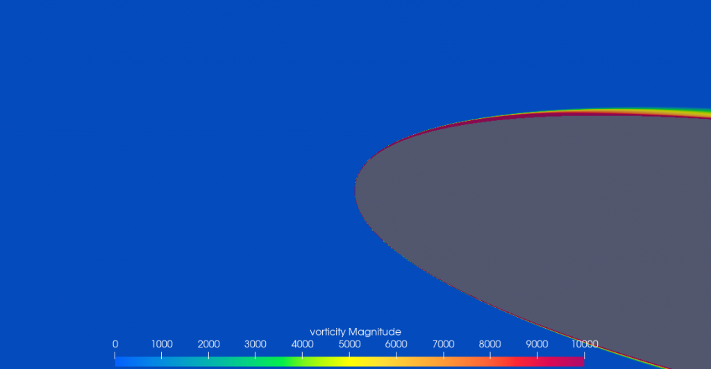
We can see vorticity in the boundary layer, where there’s shear flow. Outside the boundary layer, the flow is irrotational.
So, what’s wrong?
The fact that the boundary layer is usually a thin region for airfoils, and that pressure gradients across the boundary layer are negligible, allows for inviscid theory to adequately predict the pressure distribution and lift on the airfoil, but fails at drag prediction, heavily dependant on friction.
However, this adequate prediction of lift does not fully explain the physics. When Bernoulli’s equation is used to explain lift, it is generally assumed that the speed is higher at the top of the airfoil and this, based on Bernoulli’s principle, determines that the pressure has to be lower. This one-way causation is not always explicitly stated, but it is implied. And this is not compatible with the physics. If we only see pressure as a consequence of high velocity, and not part of the cause, how could we correctly explain how the high velocity got there in the first place?
Longer paths and equal transit times
This is another widespread explanation for lift. This explanation assumes a more convex upper surface and that the fluid parcels, that split at the leading edge, have to meet up again in the trailing edge. The conclusion that follows is that the fluid parcel along the upper surface has to travel faster.
Truth is that not only there’s no physical reason for this to be the case, but also empirical evidence shows that this is not. As a matter of fact, due to the no-slip condition, the time it takes for the parcels to traverse the airfoil tends to infinity the closer to the wall they are.
We can also refute this hypothesis using CFD. As we can see in the next animation, the fluid parcels over the airfoil are accelerated and reach the trailing edge faster. The two fluid parcels closer to the airfoil, that are in close proximity when reaching the leading edge, end up displaced from each other downstream.
We can also clearly see in the animation that the parcels passing over the airfoil are accelerated, while those passing under are slowed down. And in both cases, the parcel closest to the wall is the slowest.
Moreover, although curvature is a common feature of airfoils, that’s not always the case, nor a necessity for lift. For instance, the NACA 0012 airfoil has zero curvature and still generates substantial lift. Furthermore, an airfoil consisting only of a camber line (no thickness) can also produce lift with zero difference in path length as we can see in these tests conducted at NASA Langley Research Center.
The Venturi effect
This explanation is also very common, and starts from the same premise as the previous explanation, the curvature of the airfoil. But in this case, the curvature is an obstacle in the passage of the fluid that the fluid avoids by pinching a streamtube as it would do in the narrowing within a Venturi tube.
The issue with this explanation is that is does not really explain how the pinching occurs, nor why it is grater over the upper surface than over the lower surface. Furthermore, this explanation leaves out the flow turning part and doesn’t explain how the pressure gradients in the vertical direction are sustained.
Low pressures
We build our intuition around the concept of relative pressure, where there are negative values, so we tend to think that in areas of low pressure there is suction. And this line of thought is negatively reinforced whenever it is explained that the upper part of the airfoil has a greater contribution to the lift as the suction is much greater there than the thrust produced at the bottom. But the reality is quite different. The pressure, even near the absolute vacuum, always points in the direction of the wall; therefore, it would be more correct to say that lift is produced by the push that the air exerts in the lower part of the airfoil, and that the upper surface contributes by pushing, not so much, in the opposite direction.

The Coanda effect
Some explanations of lift focus on the exchange of momentum between the fluid and the airfoil; the airfoil deflects the air downward and thus imparts a downward momentum, which is balanced by an upward force air exerts on the airfoil. The angle of attack together with the airfoil curvature —if any—, saves most from explaining in detail how the air is deflected downwards by the lower part of the airfoil. But the air is also deflected at the upper part of the airfoil, so the Coandă effect is brought up to explain the fact that the current lines follow the curvature of the profile in its upper convex part.
But the truth is that the effect described by Coandă (1936) has more to do with the tendency of a jet, with a higher total pressure than the surrounding fluid, to attach to an adjacent surface. This is a result of the jet’s entrainment of surrounding fluid and restrictions imposed on the flow pattern by conservation of mass. In the airfoil case, there’s no entrainment and flow attachment is basically the absence of boundary layer separation.
We covered briefly a few of the most common misconception, but I invite you to check McLean’s book (2012) for a more detailed analysis.
Basic explanation of lift on an airfoil
A proper explanation of lift should not treat the velocity field and the pressure field separately. The cause-and-effect relationship is reciprocal; thus, an explanation based on downward turning alone or on Bernoulli alone would be incomplete.
The airfoil can impart a downward force to the flow via a combination of shape and angle of attack. As a result, part of the flow is accelerated and deflected downward in accordance with Newton’s second law. At the same time, the air pushes back with an equal and opposite force —lift—. In a steady flow this sequence is not linear; all interactions are reciprocal and simultaneous.
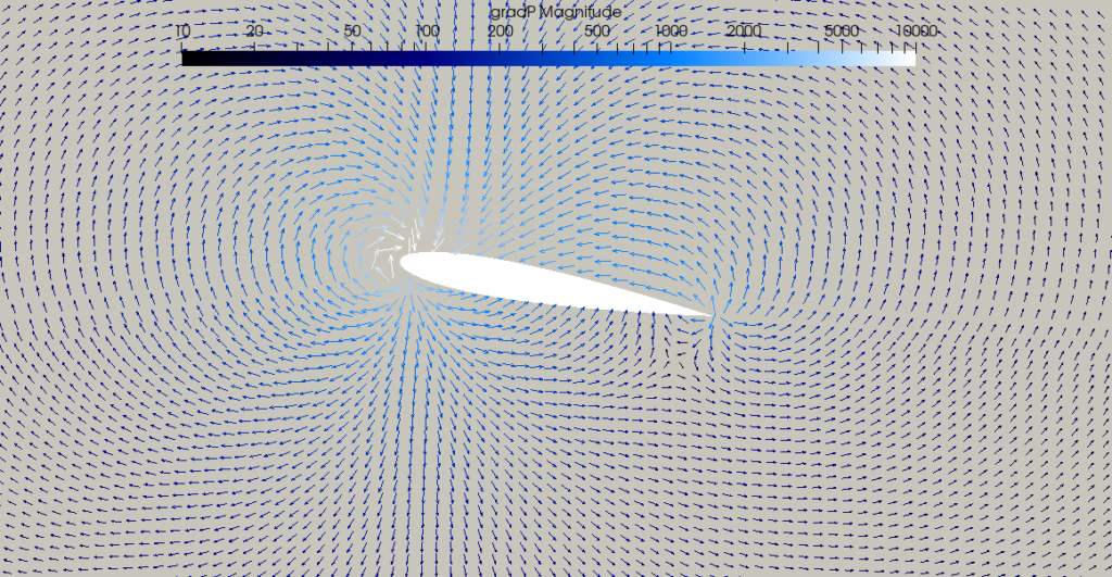
While near the walls the flow is forced to follow the contours the airfoil, a little bit further away the distribution of pressure is determined by the interaction with the velocity field. We can see that in the following figure that shows the pressure gradient $\nabla p$ overlaid on top of the velocity field $\bf{V}$.
Note: we are actually plotting the negative of the pressure gradient, so that the arrows point from the high pressure regions to the low pressure regions.
In the figure we can nicely see the interaction between the pressure field and the velocity field: how the pressure exerts a force in directions perpendicular to the isobars and how that force causes the air to accelerate in the direction of these forces. But this interaction is reciprocal as the pressure field is only sustained as long as the air resists this acceleration, i.e., it has inertia.
…with a little help from the momentum equation
This mutual interaction follows Newton’s laws of motion. It might help to visualise this laws as applied to fluid flows —the momentum equation:
$$ \rho \frac{\partial \mathbf{V}}{\partial t} + \rho (\mathbf{V} \cdot \nabla)\mathbf{V} = – \nabla p + \rho \mathbf{g} + \mu \nabla^2\mathbf{V} $$
where the first term in the temporal derivative, which we can ignore steady state; the second term is the convective acceleration —the changes in velocity we see in the figures—; the next term is the pressure gradient, followed by the body force term; and the last term, the diffusion term.
Some of the terms we can ignore straightaway, e.g., the temporal derivative —we are assuming steady state flow—, and the body force term —changes in potential energy due to gravity are negligible—. Others, like the diffusion term, only outside the boundary layer and wake, were we have irrotational, inviscid flow. Simplifying, we would therefore have on the left the convective acceleration, and on the right the pressure gradient. But do not interpret, from the way we have written the equation, that somehow $ \mathbf{V} = f(p) $. This is not at all the case. And this is evident from the way computers solve these non-linear, velocity-pressure linked equations. A great example is the SIMPLE algorithm. The solution strategy can be summarised as follows:
- Initial guess field variables.
- Solve the discretised momentum equations.
- Solve the pressure correction equation.
- Correct pressure and velocities.
- Solve all other discretised transport equations.
The steps 2 to 5 are repeated until convergence of the velocity and pressure fields.
Conclusion
As McLean (2018) also concludes, fluid flows in general are inherently complex, so the goal of a qualitative explanation should be that of describing and explaining the phenomena, which I hope to have achieved in this article by showing that pressure and velocity go hand in hand, interacting on a reciprocal basis.
References
Anderson, J. D. (2011). Fundamentals of Aerodynamics (5th ed. in SI Units). Singapore: McGraw-Hill.
Coandă, H. (1936). Device for Deflecting a Stream of Elastic Fluid Projected into an Elastic Fluid. (US Patent No. 2,052,869). USPTO.
Denker, J. S. (2005). 3. Airfoils and Airflow. [online] Av8n.com.
McLean, J. D. (2012). Understanding aerodynamics: Arguing from the real physics (1st ed.). Chichester: Wiley.
McLean, J. D. (2018). Aerodynamic Lift, Part 2: A Comprehensive Physical Explanation. The Physics Teacher, 56(8), pp.521-524.
Regis, E. (2020). No One Can Explain Why Planes Stay in the Air. [online] Scientific American.
Versteeg, H. K., & Malalasekera, W. (2007). An introduction to computational fluid dynamics: The finite volume method (2nd ed.). Pearson Education Ltd.
White, F. M. (2011). Fluid mechanics (7th ed). New York, NY: McGraw-Hill.
About Doug McLean
As I have indicated above, most of the explanation related to lift is taken from Doug McLean’s book. McLean, a retired Boeing Technical Fellow, who addresses in his book real aerodynamic situations through intuitive physical interpretations and explanations, debunking commonly held misconceptions and interpretations, and building upon the contrasts provided by wrong explanations to strengthen understanding of the right ones. The first time I heard of him was through a talk he gave on Common Misconceptions in Aerodynamics at the University of Michigan, which I leave here below, and which I highly recommend to any of you interested in understanding aerodynamics.