
2D NACA 0012 airfoil validation
This is part one of a two article series on lift in 2D which uses the NACA 0012 airfoil to illustrate some concepts related to lift. The purpose of this validation is to compare our CFD results against known data to certify that we reproduce the physics correctly. Since we will rely on these data to draw conclusions in part two of this series, being able to trust the results of our model is vital.
The reference validation case is available through NASA Langley Turbulence Modeling Resource (TMR) website, while detailed results have been reported through various papers such as Diskin et al. (2015).
Contents
Setup
Here we will give only a brief outline of the case setup; for more details you can download the finest mesh case at the end of this post, here.
Grid
NASA makes available several grids used in their verification and validation studies. Among the available options, I have opted for the Family II of structured grids, from size 225 x 64 to size 1793 x 513. The grids have been generated such that the airfoil closes at chord = 1 with a sharp trailing edge. In all available grids, the farfield extends about 500c.
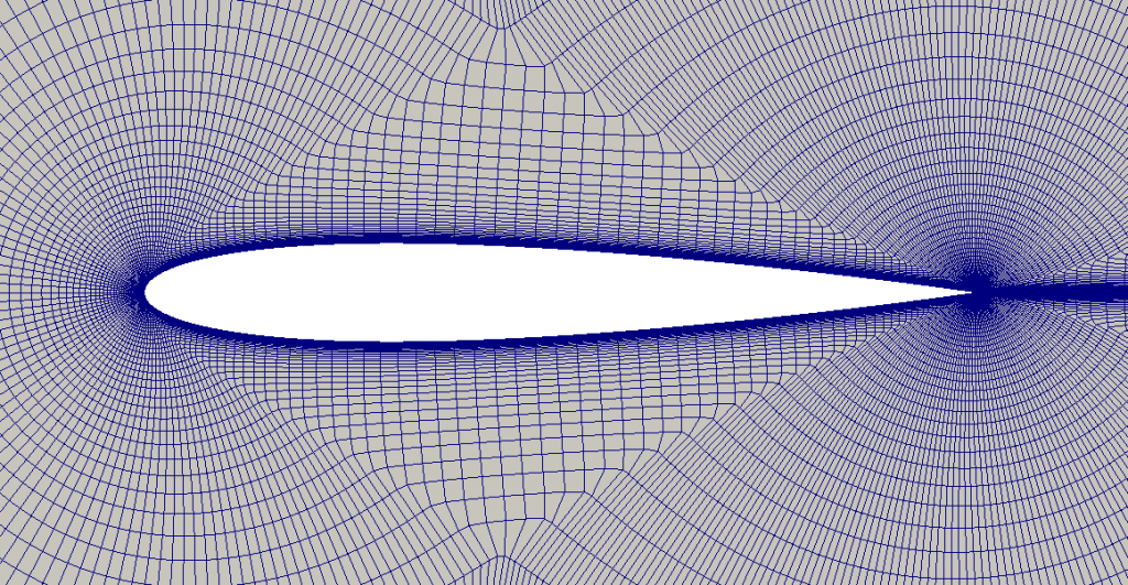
The minimum length —after scaling— at the wall is 7 x 10⁻⁷ and average stretching rate normal to the wall is ~1.02 for the points near the wall. As a result, the grid contains approximately 1 million cell.
The structured PLOT3D grids can be easily converted to OpenFOAM format with the plot3dToFoam tool.
Boundary conditions
I’ll be using the results from Diskin et al. (2015) and the TME website as reference for this case. There, we get that the conditions for the case are M = 0.15, Reynolds number per chord is Re = 6 million, alpha = 10 deg, reference temperature = 540 R. The Prandtl number Pr is taken to be constant at 0.72, while the turbulent Prandtl number Prt is taken to be constant at 0.9. The heat capacity ratio ($\gamma$) is 1.4.
The conditions above states are given for nondimensional CFD codes such as CFL3D or FUN3D. That’s not the case for OpenFOAM, so the conditions need to be translated. Firstly, we convert the reference temperature from Imperial to SI (540 R = 300 K). Secondly, once we know temperature, we can compute the speed of sound as
$$ a = \sqrt{\gamma R T} $$
where $R$ is the specific gas constant (287.058 J⋅kg−1⋅K−1 for dry air). As a result we get a speed of sound of $a$ = 347.2 m/s. Thirdly, now we can use the Mach number to get the flow velocity, $U_\infty$ = 52.08 m/s. Fourthly, we can get additional dry air properties such as kinematic viscosity $\nu_\infty$ = 15.68 x 10⁻⁶ m2/s. Finally, we can obtain the airfoil chord from Reynolds number, air velocity, and kinematic viscosity as
$$ L = \frac{\nu_\infty Re}{U_\infty} $$
which results in a chord of L = 1.80645 m. Therefore, the grid has to be scaled.
On the other hand, in the farfield we have also the following conditions:
$$ \tilde{\nu}_\rm{farfield} = 3\nu_\infty $$
$$ \nu_{t,\rm{farfield}} = 0.210438\nu_\infty $$
OpenFOAM
The following table summarises the boundary conditions used in OpenFOAM (front and back are of the empty type).
| airfoil | farfield | |
| U | fixedValue uniform (0 0) | freestreamVelocity* freestreamValue 52.08*(cos(10°) sin(10°)) |
| p | zeroGradient | freestreamPressure* freestreamValue 101360.2 |
| nuTilda | fixedValue uniform 0 | freestream* freestreamValue 47.04e-6 |
| nut | nutLowReWallFunction uniform 0 | freestream* freestreamValue 3.299668e-6 |
| T | zeroGradient | freestream* freestreamValue 300 |
| alphat | alphatWallFunction Prt 0.9 | calculated |
*The freestream, freestreamPressure, and freestreamVelocity boundary conditions inherit from inletOutlet and outletInlet. Those boundary conditions switch the mode of operation between fixed (free stream) value and zero gradient based on the sign of the flux.
Sutherland’s law
NASA repeats through several sections in their website —like here— that in their codes, dynamic viscosity is computed using Sutherland’s law,
$$ \mu = \mu_0 \left( \frac{T}{T_0} \right)^{3/2} \left( \frac{T_0 + S}{T + S} \right) $$
were $S$ it the Sutherland temperature (110.4 K). In OpenFOAM, Sutherland’s law is written differently, as
$$ \mu = \frac{A_s \sqrt{T}}{1 + S/T} $$
Comparing the formulas above, we can write the constant as:
$$ A_s = \frac{\mu_0}{T_0^{3/2}} (T_0 + S) $$
were $\mu_0$ = 1.176 x 10⁻⁵ kg⋅m-1⋅s-1, $T_0$ = 273.15 K, and $S$ = 110.4 K. Thus, $A_s$ = 1.458 x 10⁻⁶ kg⋅m-1⋅s-1⋅K-1/2.
We can enable Sutherland’s law in the thermophysicalProperties dictionary.
Note: I compiled a new implementation of the Sutherland transport model which uses the Prandtl number to calculate thermal conductivity. The code is accessible in GitHub: https://github.com/pfsq/mySutherland
The Spalart-Allmaras turbulence model
Ludwig Prandtl pointed out that certain fluid flows could be divided into a thin viscous layer —boundary layer— near surfaces and an effectively inviscid outer layer. In the inviscid outer layer the Euler and Bernoulli equations apply. But in boundary layers, which are predominantly turbulent, the assumptions taken by Euler and Bernoulli do not hold. Some empirical equations were developed for predicting the turbulent over a flat plate, yet the turbulent flow over arbitrarily shaped bodies still involves the solution of the continuity, momentum, and energy equations along with some model of the turbulence. Philippe Spalart and Steve Allmaras. proposed one of such models.
The one uncontroversial fact about turbulence is that it is the most complicated kind of fluid motion.
Peter Bradshaw, Imperial College
The Spalart-Allmaras model is a linear eddy viscosity that solves one additional transport equation. Because it is computationally cheaper, it is used in many codes and, for many flows, its performance is comparable to that of many more complicated models.
Many variants of the model have been proposed since its introduction in the early 1990s. Specifically, OpenFOAM’s implementation of the model ignores the $f_{t2}$ laminar suppression term; otherwise, the model is identical to the standard version. But as long as the simulation is at a relatively high Reynolds and $\tilde{\nu}_\rm{farfield} = 3\nu_\infty$, ignoring the $f_{t2}$ term should make little difference, as is the case here. In any case —for the inquiring eye— I have implemented the standard version of the Spalart-Allmaras model by reintroducing the $f_{t2}$ term: https://github.com/pfsq/standardSA; unsurprisingly, the results are almost identical.
In Diskin et al. (2015), the codes FUN3D and TAU use the SA-neg variant of the SA turbulence model that admits negative values of the Spalart turbulence variable, while for positive values of $\tilde{\nu}$ the model remains identical to the standard version. In any case, this variant should provide negligible differences in most cases.
Note: older versions of OpenFOAM (v2.x and older) need changes to the turbulence models to match the definitions found in NASA’s website.
Numerical schemes
The solutions from all three codes in Diskin et al. (2015) are second order accurate via a MUSCL scheme. Although these schemes are also available in OpenFOAM, I was getting unstable simulations, so I used linearUpwind instead, for velocity, energy, and turbulence, and linear for the rest. As with MUSCL, both schemes are second order accurate discretizations of the advective terms.
Since the solution was initiated with the coarsest mesh and then each successive solution mapped to the next grid level, it was not necessary to start with lower order schemes.
Linear solvers
I used the PCG solver with FDIC preconditioner for pressure —GAMG was very unstable— and PBiCGStab with DILU preconditioner for the asymmetric matrices.
For asymmetric matrices, we set a tight tolerance of less than 1e-10, while for pressure —as it is more expensive to calculate— we run with a relative tolerance of 0.001.
Solution
The cases were solved with a compressible solver, rhoSimpleFoam, and with the standard Spalart-Allmaras turbulence model. Each was iterated for 5000 steps —except for the finest mesh, which required 10000—, reaching convergence to at least 4 significant digits.
Convergence of residuals and variables of interest
Residuals go down nicely, although turbulence and energy seem to reach a lower limit at 1e-4 and 1e-7, respectively.
Drag, lift, and moment coefficients reach an asymptotic value after several thousand iterations. The variation over the last 2000 iterations is minimal, and although U residuals were still show a decreasing trend, I considered convergence to be sufficient for this analysis.
*Click on the legend to display or hide the coefficients.
Grid convergence behaviour
The following charts illustrate grid convergence for the lift, drag, and moment coefficients. The finest grid I was able to run in OpenFOAM was two levels coarser than the finest mesh available. At the finest meshes, OpenFOAM simulation was very unstable, which I believe is related to the extremely high aspect ratios of these meshes in the wake region.
We can see that lift and drag coefficients in OpenFOAM do not exhibit a clear order property: the lift coefficient first increases, then decrease on the finer grids (the other way around in the case of drag coefficient). In all, a convergence behaviour that is very different from that observed in the study by Diskin et al. (2015).
On the contrary, this is not the case for these other two coefficients, the viscous drag coefficient and the moment coefficient. Here the trend is very clear and the values are very close to the reference ones.
Diskin et al. (2015) show that variations in discretization schemes have a great influence on the evolution of the variables towards convergence, but that the value towards which they should tend as the mesh is finer, should be the same.
In any case, results for the finest mesh run in OpenFOAM are < 0.7 % off target for the main aerodynamic coefficients—which is a quite good approximation— the largest deviation being pressure drag at 1.2 %. Although from the convergence graphs, the trend would seem to indicate that the lift and drag values might deviate somewhat more from our target. These differences could be due to several factors, namely discretization errors, iterative convergence differences, boundary condition differences, and/or possible code-to-code implementation-detail differences (Rumsey, 2018).
| Ladson (1988)* | Rumsey (2019) | OpenFOAM | Relative % | |
|---|---|---|---|---|
| CL | 1.0586 – 1.0672 | 1.0909 – 1.0911 | 1.090171 | -0.09% – -0.07% |
| CD | 0.01149 – 0.01191 | 0.01227 – 0.012275 | 0.01234813 | +0.60% – +0.64% |
| CDp | – | 0.00606 – 0.00607 | 0.006132005 | +1.02% – +1.19% |
| CDv | – | 0.006205 – 0.006206 | 0.006217443 | +0.18% – +0.20% |
| Cm | – | 0.00676 – 0.0068 | 0.006799703 | +0.00% – +0.59% |
*It is very difficult to get fully two-dimensional conditions in experiments, specially as the angle of attack increases. So, this data should be considered with that in mind, and is provided here solely as reference. Further comparisons of results are done only against other CFD codes.
Note: In the Supporting material section I provide everything necessary for anyone to replicate this validation study. Feel free to download the material and give me your feedback on the subject.
Surface pressure and skin friction
To understand where the differences are with respect to the reference models, we will compare values on the surface of the airfoil and along several lines in the vicinity of the airfoil.
The solutions of surface pressure and skin friction coefficients are almost indistinguishable in moderately zoomed views. We have to zoom-in very close to see the biggest differences. For instance, the OpenFOAM solution shows a smaller peak minimum pressure and a larger peak maximum skin friction. As a result, when we integrate this small variations over the whole surface, they will add up to the differences seen in lift and drag coefficients. Moreover, the differences seem to be distributed along the profile, which is why the moment coefficient is practically identical to the reference values as differences on both sides of the centre of rotation are balanced.
Various profiles along different lines
To further evaluate the results of our model, we will also compare the results of some variables along several lines in the vicinity of the trailing edge.
The curves for the reference cases are taken from the finest mesh. In most situations, the difference with the results of coarser meshes is small, and I omit them so as not to overload the plots. On the other hand, for the profile along x/c=10, the difference between meshes is very significant, so I include in a different stroke the results for the mesh two levels coarser.
Pressure coefficient
We find the most noticeable differences in the pressure profile in the area close to the wall. As we can see in the following two graphs, the pressure profile, as we move away from the surface, approaches the value calculated by the other codes, more so in the lower part of the airfoil than in the upper part.
Just behind the trailing edge, the profiles begin to be indistinguishable from each other.
As mentioned before, the differences are mainly in the vicinity of the surface. In their study, Diskin et al. (2015) show that mesh resolution is an important factor here, and that a fine mesh is needed to accurately represent the local solution.
Horizontal velocity component
The horizontal velocity component u profile near the trailing edge is almost identical in all codes.
We find the largest variation in horizontal velocity in the wake far from the airfoil, at x = 10, where the resolution of the coarser mesh does not allow to properly resolver the wake. For this reason, I also include here the results obtained with FUN3D and CFL3D for the equivalent mesh —dash dot line.
What I find remarkable in the previous plot is that, although the profile is similar in magnitude and shape, in OpenFOAM we don’t see an overflow to then return to the value in the far field, i.e., u/aref never exceeds 0.148.
Vertical velocity component
The solution calculated by OpenFOAM, also can hardly be distinguished from the ones obtained by means of FUN3D and TAU, and only in the upper region the result of CFL3D is slightly different.
As with the horizontal velocity component, the vertical component in the wake is influenced by the resolution of the mesh in the region. The results, for this profile, are also comparable to those of the equivalent mesh computed by the other codes.
Eddy viscosity
Eddy viscosity is also practically identical between codes. The differences between OpenFOAM and the other codes are mainly when approaching 0. FUN3D and TAU use the SA-neg variant which allows negative values of the Spalart turbulence variable, while clipping $\nu_t$ at 0. There are also differences in the discretization schemes that influence the behaviour of the variable near the transition to zero.
It is clear that the resolution of the mesh is decisive when it comes to accurately resolving the wake. We have already seen this in the other profiles, and in the case of eddy viscosity it is the same.
Concluding remarks
The correlation with the reference simulations is very good. The difference is less than 1% with respect to the codes used by NASA, and the differences can be attributed to various factors such as differences in divergence schemes, the implementation of codes or variations in imposed boundary conditions.
On the other hand, grid convergence is something we should investigate in more detail. Diskin et al., when faced with this phenomenon, they attributed it to the resolution of the mesh near the trailing edge, and solved this issue with family II of grids, which is the family of grids we have used in this study.
Stay tuned, for I will shortly be publishing an article based on this one which I hope will be just as interesting to all of you.
References
Allmaras, S., Johnson, F., & Spalart, P. (2012). Modifications and Clarifications for the Implementation of the Spalart-Allmaras Turbulence Model. In Seventh International Conference on Computational Fluid Dynamics (ICCFD7). Big Island, Hawaii.
Diskin, B., Thomas, J., Rumsey, C. L., & Schwoeppe, A. (2015). Grid Convergence for Turbulent Flows (Invited). 53rd AIAA Aerospace Sciences Meeting. Presented at the 53rd AIAA Aerospace Sciences Meeting, Kissimmee, Florida.
Ladson, C. (1988). Effects of Independent Variation of Mach and Reynolds Numbers on the Low-Speed Aerodynamic Characteristics of the NACA 0012 Airfoil Section. NASA TM 4074. Hampton, Virginia: NASA Langley Research Center.
Rumsey, C. (2018). 2D NACA 0012 Airfoil Validation – SA Model Results. Retrieved 7 December 2019, from https://turbmodels.larc.nasa.gov/naca0012_val_sa.html
Rumsey, C. (2019). 2D NACA 0012 Airfoil Validation for Turbulence Model Numerical Analysis – SA Model Results without Point Vortex BC. Retrieved 7 December 2019, from https://turbmodels.larc.nasa.gov/naca0012numerics_val_sa_withoutpv.html
Appendix: supporting material
If you would like to run this model on your own, and help me verify the model, here you have the links to the sources: