Simulating the tire contact patch region

Wheels and tires could be regarded as some of the trickiest components to model and get right in a CFD simulation. This is because —unlike the sprung parts of the car— the wheels are in constant rotation with respect to a reference frame established on the vehicle itself. Furthermore, the flow around the wheel area is highly unsteady and complex with many regions prone to separation.

A particularly difficult area to model is the contact patch between the wheel and the ground. This region is the topic of this article.

Contact patch

In the case of a solid cylinder, the contact between the cylindrical surface and the flat ground would be through a contact line. However, in the case of a wheel this contact is a surface—contact patch—, the size of which depends on the stiffness characteristics and the load of the tire.

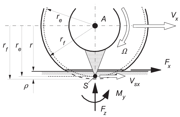
The tire, due to the fact that it is subjected to a load —weight of the vehicle—, has radial deflection $\rho$. This causes the wheel to deform and lose its circular shape—the side walls bulge out, the pattern is squeezed and distorted, and the tire connects with the ground forming a contact patch (Hobeika & Sebben, 2018). Replicating the deformed shape is usually omitted in CFD simulations, although the contact patch is still considered.

All this results in a smaller effective radius (free rolling) which defines a slip circle. At free rolling, the longitudinal velocity of point S —which lies on the slip circle—, at its lowest position, becomes equal to zero. We have at free rolling on a flat road a velocity of the wheel centre in the forward direction defined as

$$ V_x = r_e \Omega $$

with $\Omega$ denoting the speed of revolution of the wheel body (Pacejka & Besselink, 2012). This reduced effective radius should be considered when defining our boundary conditions.

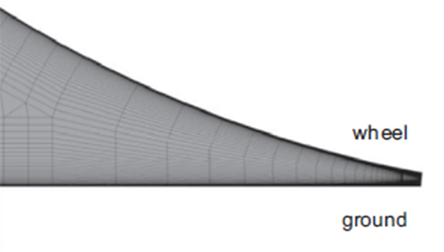
But let’s do not deviate from the subject: simulating the contact patch region. Since meshing the contact zone between the ground and tyre produces cells with a lot of skewness —acute junction—, it is common to introduce a step around the perimeter of the contact patch. But I found a couple of other choices as we’ll see below.

Mesh

I have created three meshes —based on the DrivAer model— to show some of the different approaches available when dealing with this tricky area:

1. defining a vertical wall with a pre-defined thickness to avoid prism cells collapsing,
2. keeping the previous vertical wall with prism-cells on the outside, but meshing the inner wedge with just tetrahedrons, and
3. defining an area close to the wheel-road contact where no prism-cells are allowed.

The three meshes can be seen in the following pictures.

• 

• 

• 

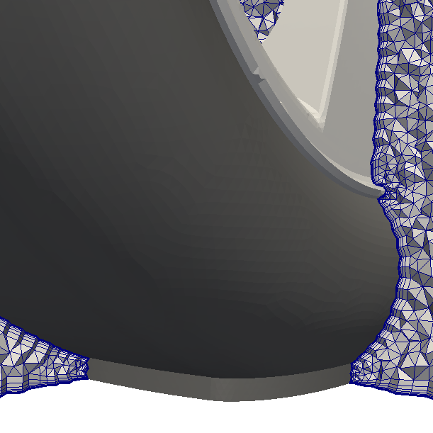
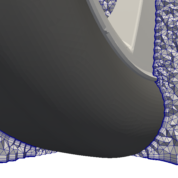
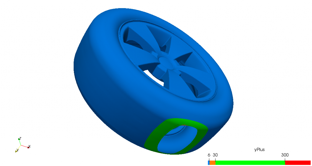
The results are relatively fine meshes with 12 prism layers and a y+ target below 6 —viscous sublayer—, adding up a total of ~9 million cells. Only in the region of the contact patch, where prism layers have been disabled, the y+ increases, although remaining within the log-law region.

A better option

For instance, structured meshers might be able to extend prism layers closer to the contact edge of the tire with the floor, merging the the two converging layers into one, as in the study conducted by Diasinos et al. (see picture below). This would be ideal, as we would be resolving the viscous sublayer all the way to the ground.

Case setup

The steady state assumption is used —as is common in industry—, with an MRF approach for modelling the rotation of the rims. For turbulence, Menter’s SST variant of the k-omega model was used. Finally, in the table you can find a list of the main boundary conditions used in the calculations.

Boundary:	inlet	outlet	farfield	wheel
p	zeroGradient	fixedValue uniform 0	zeroGradient	zeroGradient
U	fixedValue uniform (30 0 0)	zeroGradient	slip	rotatingWallVelocity omega 96.774
k	fixedValue uniform 0.135	zeroGradient	zeroGradient	kLowReWallFunction* uniform 0.135
omega	fixedValue uniform 893.819	zeroGradient	zeroGradient	omegaWallFunction uniform 893.819
nut	calculated uniform 0	calculated uniform 0	calculated uniform 0	nutUSpaldingWallFunction uniform 1e-10

*For the region of the tire were no prism layers have been grown, we used the kqRWallFunction.

Results

Both cases were iterated until the variable of interest —drag coefficient— reached an asymptotic value. The results —based on the last 500 iterations— are shown in the following table.

Case	Drag coefficient
Without contact patch step	0.4954 ± 0.0002
With contact patch step	0.4582 ± 0.0001

Drag of the model with step was approximately 7.5 % less than that obtained without step. A smaller difference compared to the 20% difference obtained by Diasinos et al. in his research between the highest and smallest step, despite their steps being relatively smaller. This smaller drag difference could be attributed to not fully resolving the boundary layer near the contact patch for the case without step, which would be essential in order to properly estimating the forces in that region, but also to the differences in tire dimensions —DrivAer tire is narrower and taller.

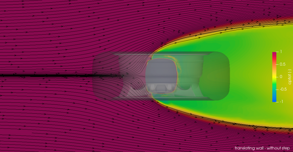
Pressure contours

• 

• 

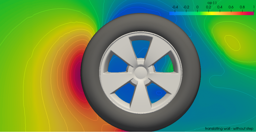
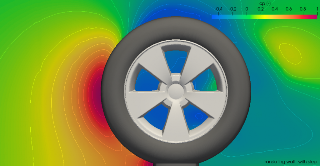
The images above show the pressure coefficient contours in a plane passing through the centre of the wheel whilst the following plot shows the pressure coefficient along the tire centre line. The curve begins on the side of the wheel exposed to the flow and the 0 coordinate has been set at the point where the step intersects with the tire —the dashed lines represent the coordinates were the step begins—, with positive arc length following the contour of the tire clockwise.

Now, in case you’re wondering how can the pressure coefficient be larger than 1, this is due to the moving boundaries transmitting energy into the flow through shear stresses in the converging boundary layers.

Clearly, the pressure along most of the upper half surface of the tire is almost identical on both models. But the lower pressure near the contact path for the model with a step weakens the jetting flow. As a result, this reduces downwash and shifts the separation point forward at the top of the wheel. This also leads to slightly higher pressures at the rear of the tyre, which once integrated result in a smaller drag.

Total pressure contours

The differences in the jetting flow and downwash can be seen in the following pictures that show the contours of coefficient of total pressure at planes normal to the freestream at x/d = 1. In the images you can tell that the downwash is somewhat stronger —though barely noticeable— when the step is not included in the model.

• 

• 

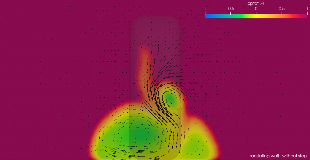
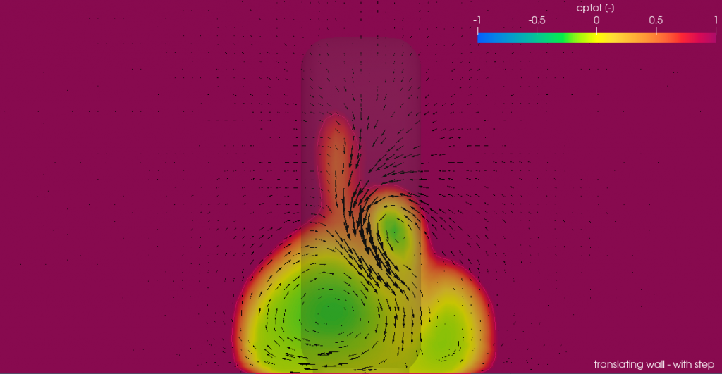
Also, the wake is wider in the case without step due to the higher pressure strengthening the jetting flow. This is also clearly visible from the top. In both images, the clip has been placed 5 mm above the ground.

• 

• 

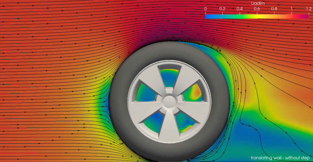
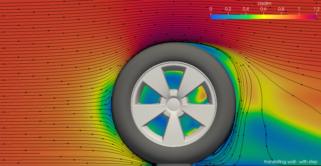
Velocity

As we saw earlier, the pressure field in the upper half of the wheel is almost the same. This leads us to think that the velocity field in that zone will be very similar as well; there are hardly any differences in the point at which the flow is detached. But the wake does vary by the influence of contact patch as we can see in the following images.

• 

• 

Conclusion

At this point you might be wondering whether simulating a tire on its own is worth your while. Because, you know, tires are usually attached to a chassis; and, either exposed as in an open-wheeler, or covered by the wheelhouse. But let me assure you, that’s not always the case…

In any case, in this article we have focused on evaluating the implications of modelling without or with step the contact patch region. This region of the wheel is always exposed, whether in Formula or conventional vehicles. Therefore, it is a delicate area, whose influence on the aerodynamics of the rest of the vehicle will spread to a greater or lesser extent depending on how the region is modelled. In Formula vehicles, mainly, the wake of the front wheel could affect the prediction of ground effect —a very important portion of the downforce—, while in conventional vehicles will vary, among other things, the prediction of the wake of the whole vehicle, and therefore the drag.

In short, a very delicate region to model that still brings engineers upside down.

References

Cavusoglu, Ö. F. (2017). Aerodynamics Around Wheels and Wheelhouses (MSc Thesis). Chalmers University of Technology, Göteborg.

Diasinos, S., Barber, T. J., & Doig, G. (2015). The effects of simplifications on isolated wheel aerodynamics. Journal of Wind Engineering and Industrial Aerodynamics, 146, 90–101.

Haag, L., Blacha, T., & Indinger, T. (2017). Experimental Investigation on the Aerodynamics of Isolated Rotating Wheels and Evaluation of Wheel Rotation Models Using Unsteady CFD. International Journal of Automotive Engineering, 8(1), 7–14.

Haag, L., Kiewat, M., Indinger, T. and Blacha, T. (2017). Numerical and Experimental Investigations of Rotating Wheel Aerodynamics on the DrivAer Model With Engine Bay Flow. Volume 1B, Symposia: Fluid Measurement and Instrumentation; Fluid Dynamics of Wind Energy; Renewable and Sustainable Energy Conversion; Energy and Process Engineering; Microfluidics and Nanofluidics; Development and Applications in Computational Fluid Dynamics; DNS/LES and Hybrid RANS/LES Methods.

Hobeika, T., & Sebben, S. (2018). CFD investigation on wheel rotation modelling. Journal of Wind Engineering and Industrial Aerodynamics, 174, 241–251.

Knowles, R. D. (2005). Monoposto Racecar Wheel Aerodynamics: Investigation of Near-Wake Structure & Supporting-Sting Interface (PhD Thesis). Cranfield Univesity.

Lew, C., Gopalaswamy, N., Shock, R., Duncan, B., & Hoch, J. (2017). Aerodynamic Simulation of a Standalone Rotating Treaded Tire. 2017-01–1551.

Pacejka, H. B., & Besselink, I. (2012). Tire and vehicle dynamics (3. ed). Amsterdam: Elsevier/Butterworth-Heinemann.

Sebben, S. (2004). Numerical Simulations of a Car Underbody: Effect of Front-Wheel Deflectors. Presented at the SAE 2004 World Congress & Exhibition.