
Physic models in STAR-CCM+ (Part IV: turbulence models)
We can find turbulence every day in almost every daily situation, whether it be smoke from a cigarette, water in a river or waterfall, the flow in boat wakes and around aircraft wing tips. Turbulent flows are characterized mainly by unsteadiness, vorticity, three-dimensionality, dissipation, wide spectrum of scales, and large mixing rates.
Turbulent flows are irregular in nature. This makes a deterministic approach to turbulence problems impossible and therefore statistical methods are used for treating turbulent flows. There are several leading computational approaches to turbulent flows and all of them fall under one of these approaches:
- Simulations, where equations are solved for a time dependent velocity field that, to some extent, represents the velocity field $\vect{U}(\vect{x},t)$, for one realization of the turbulent flow.
- Turbulence models, where equations are solved for some mean quantities $\langle \vect{U} \rangle$, $\langle u_iu_j \rangle$, and $\varepsilon$.
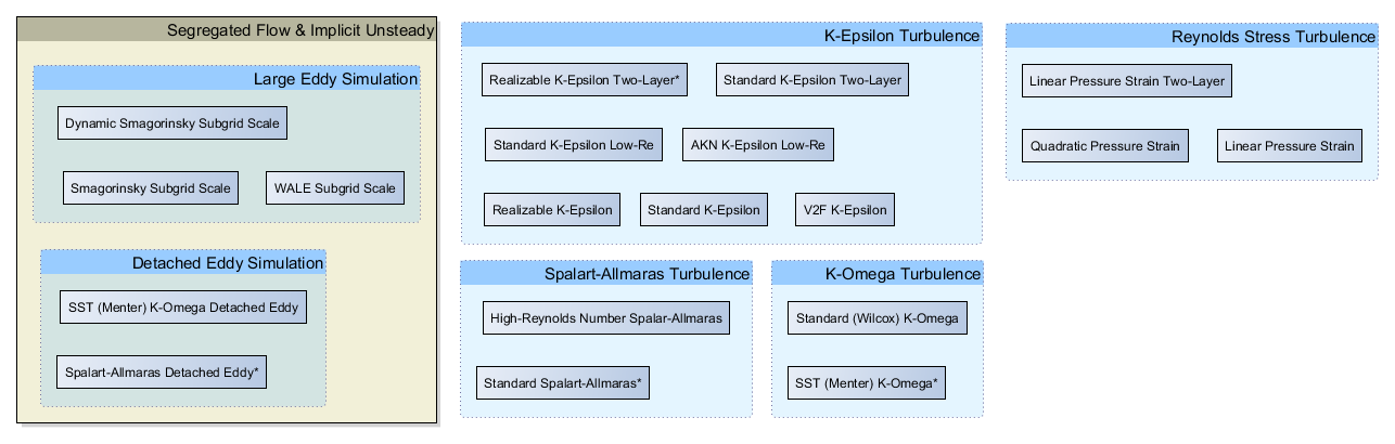
In STAR-CCM+ the available approaches to modelling turbulence are:
- Models that give closure of the Reynolds-Averaged Navier-Stokes (RANS) equations.
- Large eddy simulation (LES).
- Detached eddy simulation (DES).
Over the years, many models have been proposed and many are currently in use. As no single turbulence model is the best for every flow simulation, it is important to follow some criteria to assess different models, such as,
- Level of description.
- Completeness.
- Cost and ease of use.
- Range of applicability.
- Accuracy.
Following comes a description of the most common approaches used today and easily found on any CFD software.
Contents
Direct numerical simulation
In DNS, the Navier-Stokes equations are solved to determine $\vect{U}(\vect{x},t)$ for one realization of the flow. Conceptually it is the simplest approach and, when it can be applied, it is unrivalled in accuracy and in the level of description provided. However, computational cost is extremely high. To an approximation, the number of floating-point operations required to perform a simulation is proportional to the product of the number of modes and the number of steps, $N^3M$ (mode-steps). The preceding results yield
$$N^3M \sim 160 {\rm Re}^3_L \approx 0.55 {\rm R}^6_\lambda,$$
showing the very steep rise with the Reynolds number.
Generally, the computational cost increases so steeply with the Reynolds number (as ${\rm R}^6_\lambda$ or ${\rm Re}^3_L$) that it is impracticable to go much higher than ${\rm R}_\lambda \sim 100$ with gigaflop computers —my Intel C2Q Q8300 peaks at 31 GFLOPS, but we may easily find recent desktop architectures, such as Haswell, exceeding 150 GFLOPS.
In Reynolds-Averaged Navier-Stokes (RANS), the Navier-Stokes equations for the instantaneous velocity and pressure fields are decomposed into a mean value and a fluctuating component. The resulting equations for the mean quantities are essentially identical to the original equations, except that an additional term now appears in the momentum transport equation, the Reynolds stress tensor:
$$ \vect{T}_t \equiv -\rho\overline{v’v’}=-\rho \begin{bmatrix}
\overline{u’u’} & \overline{u’v’} & \overline{u’w’} \\
\overline{u’v’} & \overline{v’v’} & \overline{v’w’} \\
\overline{u’w’} & \overline{v’w’} & \overline{w’w’} \end{bmatrix}$$
To model this Reynolds stress tensor in terms of the mean flow quantities, two basic approaches are available: turbulent-viscosity models and Reynolds-stress models.
Turbulent-viscosity models
These models use the concept of a turbulent viscosity $\mu_t$ to model the Reynolds stress tensor as a function of mean flow quantities.
Classes of turbulence models available in STAR-CCM+ include Spalart-Allmaras, K-Epsilon and K-Omega models.
K-Epsilon models
Introduced in 1972 by Jones and Launder [4], the K-Epsilon model belongs to the class of two equation models, in which model transportation equations are solved for two turbulence quantities. It is the most widely used complete turbulence model, and it is incorporated in most commercial CFD codes.
The K-Epsilon model consists of the model transportation equation for $k$
$$ \frac{\bar{\rm D}k}{\bar{\rm D}t} = \nabla\cdot \left( \frac{\nu_T}{\sigma_k} \nabla k \right) + \mathcal{P} – \varepsilon, $$
the model transportation equation for $\varepsilon$
$$ \frac{\bar{\rm D}\varepsilon}{\bar{\rm D}t} = \nabla\cdot \left( \frac{\nu_t}{\sigma_\varepsilon}\nabla\varepsilon \right) + C_{\varepsilon 1}\frac{\mathcal{P}\varepsilon}{k} – C_{\varepsilon 2}\frac{\varepsilon^2}{k}, $$
which is empirical, and the specification of the turbulent viscosity as
$$ \nu_T = C_\mu k^2/\varepsilon. $$
It is somewhat a semi-empirical model, mainly because the modelled transport equation for dissipation used in the model depends on phenomenological considerations and empiricism.
Standard K-Epsilon
This is the de facto standard version of the two-equation model that involves transport equations for the turbulent kinetic energy $k$ and its dissipation rate $\varepsilon$.
Standard K-Epsilon Two-Layer
This model combines the Standard K-Epsilon model with the two-layer approach, which allow the K-Epsilon model to be applied in the sublayer.
In the layer next to the wall, the turbulent dissipation rate $\varepsilon$ and the turbulent viscosity $\mu$, are specified as functions of wall distance. The values of $\varepsilon$ specified in the near-wall layer are blended smoothly with the values computed from solving the transport equation far from the wall.
Standard K-Epsilon Low-Re
This model has identical coefficients to the Standard K-Epsilon model, but provides more damping functions. These functions let it be applied in the viscous-affected regions near walls.
Realizable K-Epsilon
Proposed by Shih et al. [5] in 1994, this model differs from the Standard K-Epsilon model in that it contains a new formulation for the turbulent viscosity and it has a new transport equation for the dissipation rate $\varepsilon$ which is derived from an exact equation for the transport of the mean-square vorticity fluctuation.
The term realizable means that the model satisfies certain mathematical constraints on the Reynolds stresses.
Realizable K-Epsilon Two-Layer*
The Realizable Two-Layer K-Epsilon model combines the Realizable K-Epsilon model with the two-layer approach. The coefficients in the model are identical, but the model gains the added flexibility of an all y+ wall treatment.
Abe-Kondoh-Nagano K-Epsilon Low-Re
It has different damping coefficients than the Standard K-Epsilon model, and uses different damping functions than the Standard Low-Reynolds Number model. It is a good choice for applications where the Reynolds numbers are low but the flow is relatively complex.
V2F K-Epsilon
The V2F K-Epsilon model is known to capture the near-wall turbulence effects more accurately. It is based on the root mean square normal velocity fluctuations $\overline{v’^2}$ as the velocity scale rather than turbulence kinetic energy $k$; thus it is capable of handling the wall region without the need for the additional damping functions because the normal velocity fluctuations are known to be quite sensitive to the presence of wall and thus are like a natural damper.
The model employs four transport equations for the closure of the RANS equations, solving two more turbulence quantities, namely the normal stress function and the elliptic function, in addition to $k$ and $\varepsilon$.
K-Omega models
There have been many two-equation models proposed and in most of them, $k$ is taken as one of the variables, with diverse choices for the second. In 1988, Wilcox [7] proposed the original K-Omega model which takes the specific dissipation rate $\omega$ ($\equiv \varepsilon/k$) as the second variable.
$$ \frac{\bar{\rm D}\omega}{\bar{\rm D}t} = \nabla\cdot \left( \frac{\nu_T}{\sigma_\omega}\nabla \omega \right) + C_{\omega 1}\frac{\mathcal{P}\omega}{k} – C_{\omega 2}\omega^2 $$
Although the specific dissipation rate $\omega$ can be thought of as the ratio of $\varepsilon$ and $k$, there are subtle differences among them. Deriving the $\omega$ equation implied by the K-Epsilon model and taking some simplifications, the result is
$$ \frac{\bar{\rm D}\omega}{\bar{\rm D}t} = \nabla\cdot \left( \frac{\nu_T}{\sigma_\omega}\nabla \omega \right) + \left( C_{\omega 1} – 1 \right) \frac{\mathcal{P}\omega}{k} – \left( C_{\omega 2} – 1 \right) \omega^2 + \frac{2\nu_T}{\sigma_\omega k}\nabla \omega \cdot \nabla k $$
which for inhomogeneous flows contains an additional term, the final term in the equation.
SST (Menter) K-Omega*
Developed by Menter [8] in 1994, the Shear Stress Transport K-Omega model takes advantage of accurate formulation of the K-Omega model in the near-wall region with the free-stream independence of the K-Epsilon model in the far field. It does so multiplying the final additional term, obtained from deriving the K-Epsilon model, by a blending function. Close to wall the damped cross-diffusion derivative term is zero (leading to the standard $\omega$ equation), whereas remote from wall the blending function is unity (corresponding to the standard $\varepsilon$ equation).
Standard (Wilcox) K-Omega
The original model proposed by Wilcox [7], it has seen most application in the aerospace industry. Therefore, it is recommended as an alternative to the Spalar-Allmaras models for similar types of applications.
Spalart-Allmaras model
Spalart-Allmaras model is a one equation model which solves a transport equation for the turbulent viscosity $\nu_T$.
The model equation is of the form
$$ \frac{\bar{\rm D}\nu_t}{\bar{\rm D}t} = \nabla \cdot \left( \frac{\nu_t}{\sigma_\nu} \nabla \nu_T \right) + S_\nu. $$
It has clear limitations as a general model but to the aerodynamic flows for which it is intended, the model has proved quite successful.
Standard Spalar-Allmaras*
This is the original model proposed by Spalart and Allmaras [9] back in 1992.
High-Reynolds Number Spalart-Allmaras
In this derivation of the model, the viscous damping within the buffer layer and viscous sublayer is not included.
Reynolds-stress models
In Reynolds-stress models, model transport equations are solved for the individual Reynolds stresses $\langle u_i u_j \rangle$ and for the dissipation $\varepsilon$ (or for another quantity, e.g., $\omega$, that provides a length or time scale of the turbulence).
The RST model carries significant computations overhead as seven additional equations (three Reynolds shear stresses, three Reynolds normal stresses, and one for dissipation) must be solved in three dimensions (as opposed to the two equations of a K-Epsilon model). There is also likely to be a penalty in the total number of iterations required to obtain a converged solution.
This model accounts for the effects of streamline curvature, swirl, rotation, and rapid changes in strain rate in a more physical manner than that by one-equation or two-equation models. So it is used for computing cyclone flows, swirling flows in combustors, rotating flow passages, and the stress-induced secondary flows in ducts.
Large-eddy simulation
In large-eddy simulation (LES), the larger three-dimensional unsteady turbulent motions are directly represented, whereas the effects of the smaller scale motions are modelled. The modelling approach combines features of RANS in part of the flow and LES in unsteady, separated regions. Because the large-scale unsteady motions are represented explicitly, LES can be expected to be more accurate and reliable than Reynolds-stress models for flows in which large-scale unsteadiness is significant.
Detached eddy simulation
Detached eddy simulation (DES) is a hybrid modelling approach that combines features of RANS simulation in some parts of the flow and LES in others. The user gets the best of both worlds: a RANS simulation in the boundary layers and an LES simulation in the unsteady separated regions.
References
[1] User Guide STAR-CCM+ Version 8.06. 2013.
[2] Dewan, A. 2011. Tackling turbulent flows in engineering. Berlin: Springer.
[3] Pope, S. B. 2009. Turbulent flows. Cambridge: Cambridge University Press.
[4] Jones, W. and Launder, B. 1972. The prediction of laminarization with a two-equation model of turbulence. International Journal of Heat and Mass Transfer, 15 (2), pp. 301–314.
[5] Shih, T., Liou, W., Shabbir, A., Yang, Z. and Zhu, J. 1994. A new k-epsilon eddy viscosity model for high Reynolds number turbulent flows: Model development and validation. NASA STI/Recon Technical Report N, 95 p. 11442.
[6] Abe, K., Kondoh, T. and Nagano, Y. 1994. A new turbulence model for predicting fluid flow and heat transfer in separating and reattaching flows—I. Flow field calculations. International Journal of Heat and Mass Transfer, 37 (1), pp. 139–151.
[7] Wilcox, D. 1988. Reassessment of the scale determining equation for advanced turbulence models. AIAA journal, 19 (2), pp. 248–251.
[8] Menter, F. R. 1994. Two-equation eddy-viscosity turbulence models for engineering applications. AIAA journal, 32 (8), pp. 1598–1605.
[9] Spalart, P. and Allmaras, S. 1992. A one-equation turbulence model for aerodynamic flows. AIAA Paper, 92-0439.