Shelby GT350R Mustang CFD simulations
It’s been a really long time since my last post as I got a new job and didn’t find time to post anything interesting. Until recently, that I came across a with the ideal geometry for a CFD simulation; the Shelby GT350R Mustang.
As have no longer access to STAR-CCM+ student’s license, and considering myself an open-source advocate. I thought it was about time to come back to OpenFOAM, but I lack the computational resources to carry out large simulations. Cloud computing seems to be the solution. I’ve known the SimScale platform for quite some time —as you can see from some of my older posts—. I did not take advantage of the free community plan for carrying out my own projects until now, although can not consider this one entirely mine, as I was not involved in the creation of the CAD geometry used for the simulations.
Contents
Shelby GT350R CAD model
The car is the 2016 Ford Shelby GT350R Mustang, introduced at the 2015 North American International Auto Show in Detroit. It is a more refined, hardcore and limited production version of the GT350; and of all the upgrades, the most interesting from the CFD standpoint is the aerodynamic package which in the R introduces a larger splitter and rear wing to help improve downforce.
Gorgeous, isn’t it?
The CAD I’m using for this simulations, by designer/engineer S. Attah, was available in GrabCAD. It seems to be no longer accessible though; a pity, because he had some very good renders of the model as it is full of detail.
Before uploading the STL file to SimScale, we have to make sure that it is intersection free and water-tight. Afterwards, as we will mesh the air domain using snappyHexMesh, it is advisable to convert the surface mesh to ensure full compatibility with the mesher. This can be achieved through the surfaceMeshConvert command.
Mesh
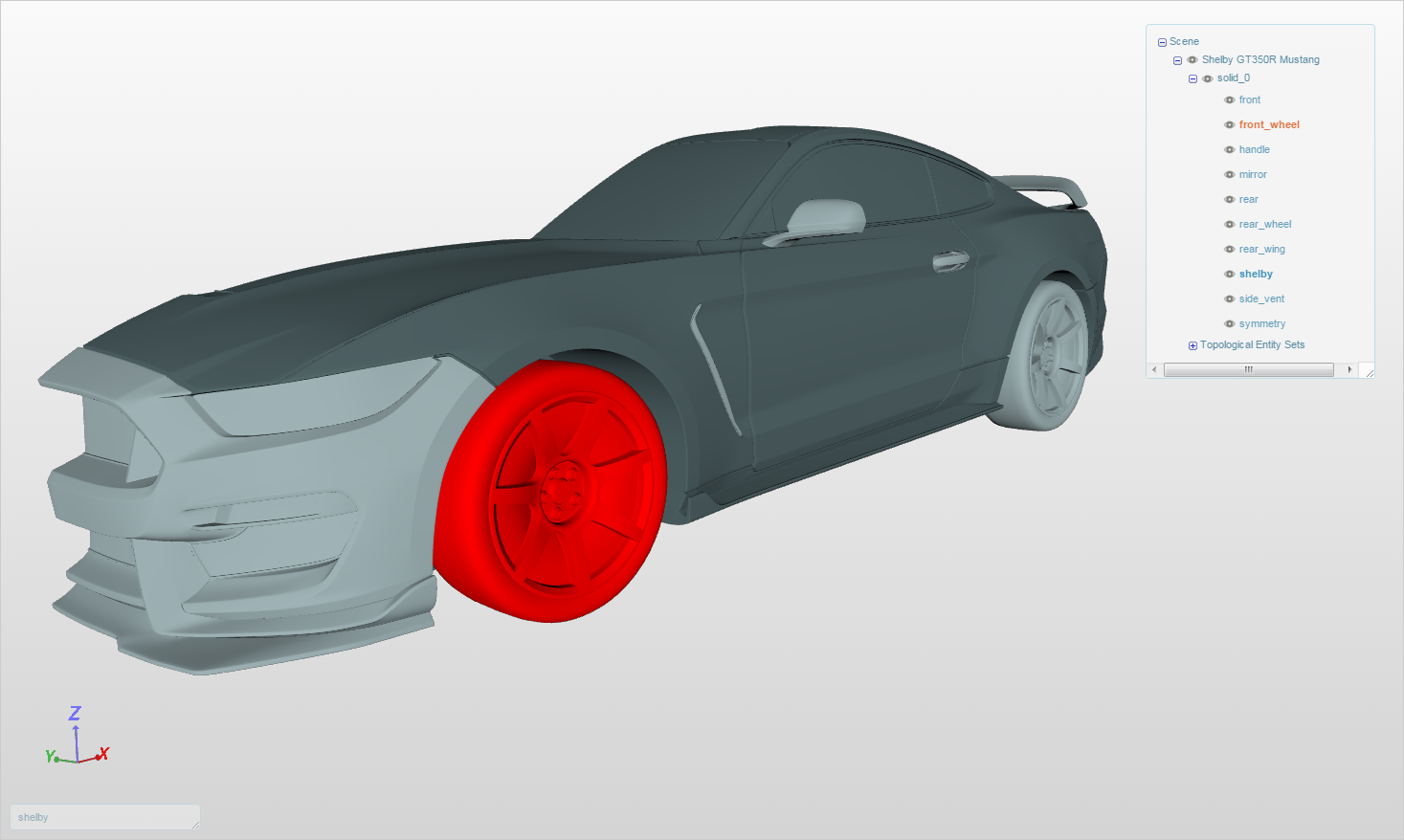
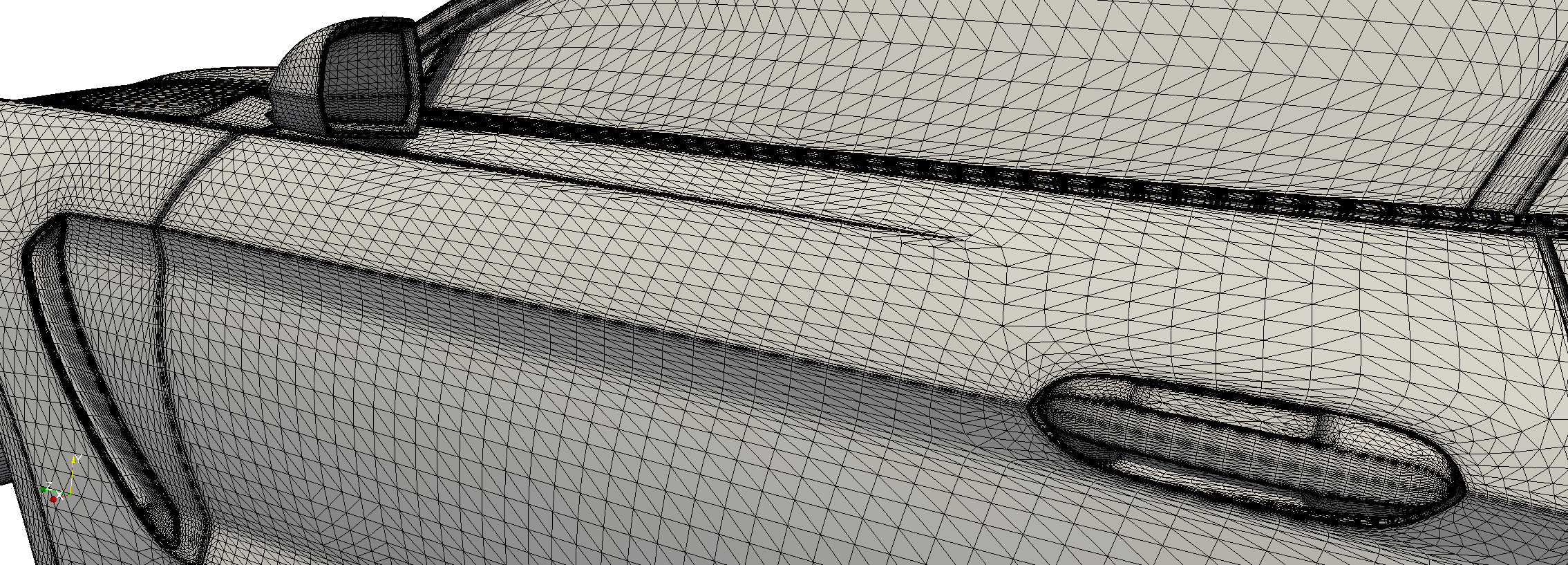
The surface was split to allow for surface refinement in selected parts of the geometry. The different sets can be seen in the following figure.
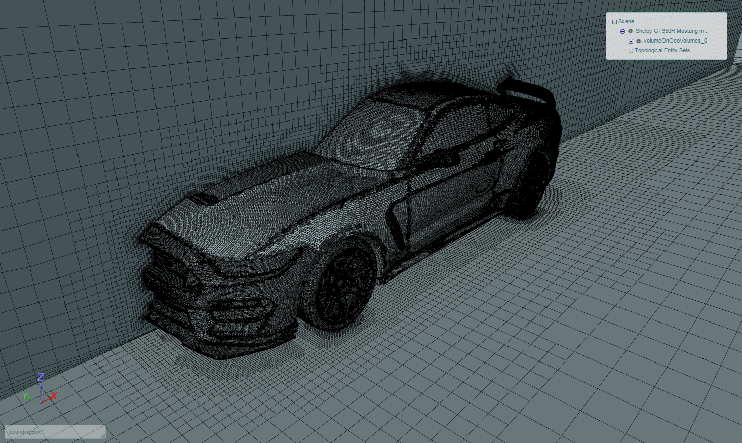
Two different meshes were generated in SimScale within an air domain of dimensions 4 × 4 × 20 m. One using the automatic settings and the other following a manual approach. In both cases, only half vehicle is considered.
The automatic mesh was set to Fine, with layer addition. The resulting mesh had 2.9 million cells.
On the other hand, the manual mesh had blocks of 1 dm3 in the farfield with refinements up to Level 7 on selected surfaces and around features adding up to 9.1 million cells.
If you click on the arrows below the picture above, you can switch the view between automatic and manual mesh. The automatic mesh is coarser near the vehicle, thus we get fewer detail on the car; but the mesh has a smaller growth rate, which implies greater resolution in the wake of the vehicle. To increase the resolution in the wake of the manual mesh, I specified a region refinement with level 4 refinement, but as you may appreciate in the figure, that didn’t work exactly the way I intended.
Simulation setup
For road vehicle external aerodynamics we can safely choose incompressible flow (Mach < 0.3, ~367 km/h). The turbulence model is the well known k-omega SST, which combines the best features of the k-omega and k-epsilon turbulence models (Dewan, 2011). The steady-state simulations are driven, under the hood, by the simpleFoam solver.
The fluid is Air, from the SimScale database with density of 1.19198 kg/m3 and kinematic viscosity of 0.0000155 m2/s.
As initial conditions, we have a uniform velocity of 35 m/s (126 km/s), turbulence kinetic energy k of 0.0459375 m2/s2, and specific turbulence dissipation ratio ω of 0.80575 /s. This values for k and ω were estimated using the turbulence online tools from CFD Online considering a low turbulence case.
Six different boundary conditions were defined for this case. A velocity inlet (35 m/s) at the inlet of the virtual wind tunnel and a pressure outlet at the exit; a symmetry plane; a moving floor (also 35 m/s); a slip wall for the side and top of the tunnel; and a no-slip wall on the car.
No kind of rotation was imposed on the wheels, as this additional pre-processing on the geometry. The geometry of the wheels is to complex as to consider the rotating walls approach acceptable, and too simple to implement MRF.
Results
Simulations were run until reaching pressure residual of 0.001 and residuals of 0.0001 for the rest. Drag and lift coefficients were also monitored up to two significant figure precision.
I downloaded the results from SimScale for further post-processing in my PC. There are some function objects and standard utilities that, as far a I know, I can only use in my local OpenFOAM installation.
By default, our simpleFoam case will save results for velocity U, turbulence kinetic energy k, turbulent viscosity νt, specific dissipation rate ω, and static pressure p. If we want additional variables, we will have to use the aforementioned function objects and standard utilities; although for some, the paraview calculator will suffice.
Pressure coefficient
Pressure distribution over the body surface is, along with shear stress distribution, the main source of aerodynamic forces and moments which we can decompose, for our interests, in drag, downforce, and aerodynamic balance.
As we usually want to compare results —whether against other vehicles or modifications we introduce on a baseline vehicle—, we must therefore resort to dimensionless quantities. And for pressure, this dimensionless quantity is the pressure coefficient
$$ C_p = \frac{p – p_\infty}{q_\infty} $$
where p∞ is the reference pressure (0 Pa) and q∞ is the dynamic pressure. We can obtain the pressure coefficient using paraview’s calculator by entering the following expression:
p/(0.5*35^2)where I used the definition of dynamic pressure in the denominator. Note that I didn’t place the density in the dynamic pressure; that’s because OpenFOAM doesn’t consider density in incompressible solvers, so that p is actually the kinematic pressure P.
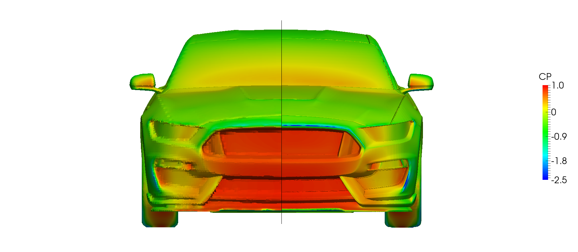
The following pictures show the dimensionless pressure distribution over the surface of the vehicle comparing, side by side, the results from the automatic and manual mesh.
It is readily apparent that the automatic mesh lacks refinement around the corners and details of the vehicle. This we can see in the lowest pressure blue areas as a consequence of the sudden change in the direction of air moving around the muscle car. Though, as we will see later on, good resolution around the object, if not accompanied by an adequate mesh for the physics involved, can also lead to non trustworthy results.
Total pressure
Closely related to static pressure, we have the concept of total pressure. This is the sum of static pressure p, dynamic pressure q, and gravitational potential energy per unit volume —we don’t usually consider gravity in most aerodynamic simulations—; that is, the sum of the mechanical energy per unit volume in a fluid.
We can get the total pressure through the ptot standard utility. Within the case folder, we just have to execute ptot -latestTime.
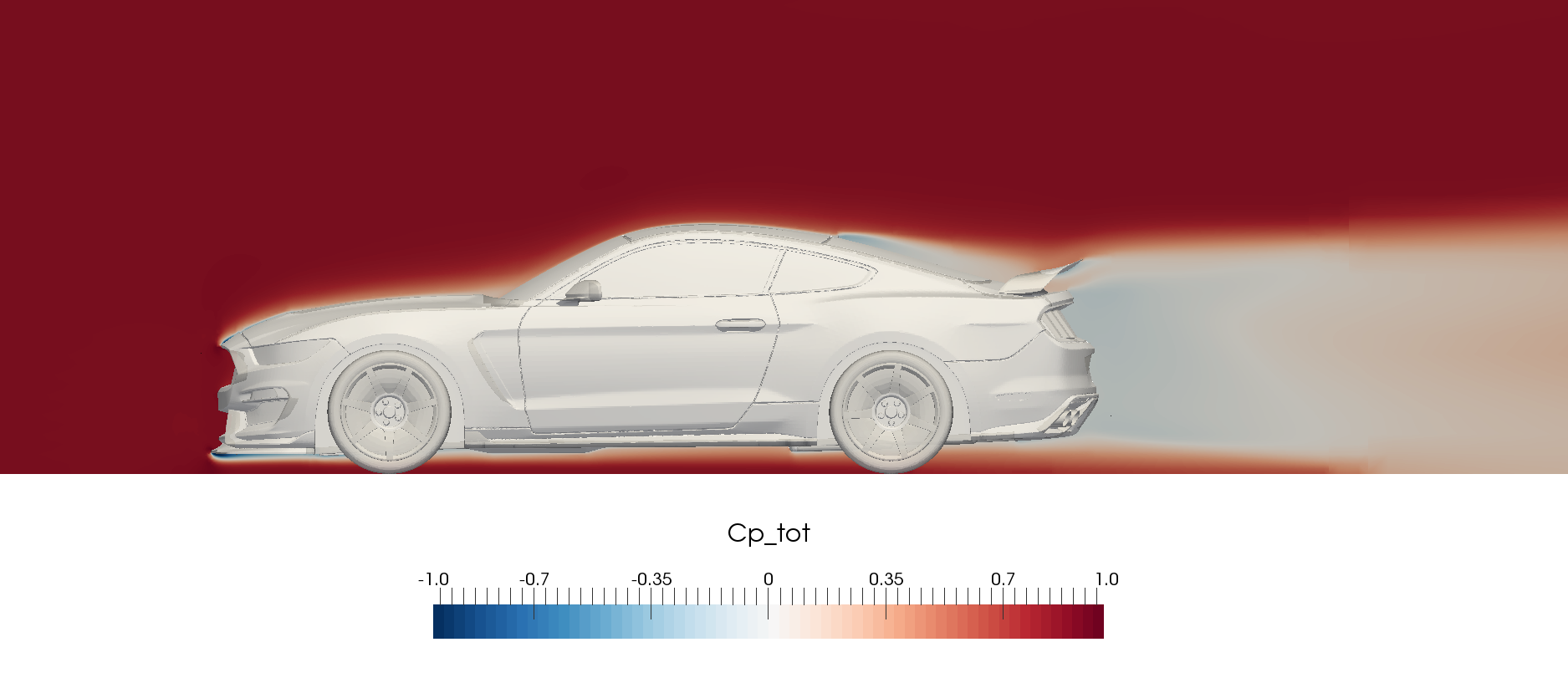
In an isentropic flow —adiabatic and reversible— the total pressure p0 at any point is a common constant value. The concept of total pressure can be applied to non-isentropic flows, as is the case; and we’ll get results as shown above where we can see the where mechanical energy losses are taking place. The effect the mesh growth rate has on the results is clearly evident. Even though the manual mesh has apparently greater resolution in the vicinity of the vehicle, the mesh is too coarse elsewhere and fails to resolve the physics downstream properly. This should raise questions about the accuracy in the estimation of the forces acting on our geometry.
Skin friction
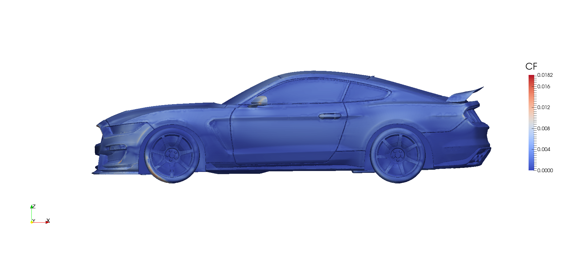
The other main source of aerodynamic force is the skin friction. The more streamlined the body, the more important the contribution of skin friction is to the total drag of the body.
We can obtain the skin friction coefficient through the wall shear stress. To compute the wall shear stress in OpenFOAM we have another standard utility wallShearStress which we use in the same fashion as ptot. We only need then to divide by the dynamic pressure q∞ to get the skin friction coefficient (remember to drop the ρ).
The skin friction coefficient might seem small when compared to pressure coefficient. But don’t be fooled, shear stress acts tangential to the surface and, when integrated over the complete body surface, can add to a significant amount of drag.
Drag and downforce
Now that we’ve gone though the sources of aerodynamic forces we can add them up and see their effect. We will keep using coefficients for the sake of comparison.
The graph shows the mean of the last tens of iterations and the standard deviation. Drag coefficient in both simulations is ~0.22; a very good result. Too good to be true.
Conclusion
Needless to say that this simulation exercise does not represent the actual aerodynamic performance of the Shelby GT350R Mustang nor is it approved or endorsed by the Ford Motor Company. Several simplifications have been taken —no rotating parts, no inlets, no outlets, and more— and the mesh lacks the required quality to resolve the physics involved to an acceptable level.
But that’s just a matter of spending more time on the pre-processing stage. Good news is that you can fork this project in SimScale and improve it. I’m looking forward to see your work.
References
Anderson, John David. 2007. Fundamentals of Aerodynamics. 4. ed. McGraw-Hill Series in Aeronautical and Aerospace Engineering. Boston: McGraw-Hill.
Dewan, Anupam. 2011. Tackling Turbulent Flows in Engineering. Berlin, Heidelberg: Springer Berlin Heidelberg.
McBeath, Simon. 2015. Competition Car Aerodynamics: A Practical Handbook. 3rd ed. Poundbury, Dorchester: Veloce Publishing.

