James Bond’s Wet Nellie

Few fictional characters are as famous as Ian Fleming’s James Bond. Proof of that is James Bond ‘s film franchise is one of the highest-grossing media franchises of all time.

The Bond films are renowned for a number of features, among which subtly modified cars, guns, and gadgets supplied by Q Branch stand out. It is precisely of one of those cars designed by Q that this article is about.

The iconic Aston Martin DB5 will surely come to mind as the most outstanding car of the entire saga. It is indisputably gorgeous and not without equipment; it includes an ejection system, twin machine guns, tire slasher, bullet-proof screen, oil slick sprayer and a long etcetera.

But let’s leave aside the DB5 and focus on the second most famous car of the British Secret Service agent.

The Lotus Esprit S1 Wet Nellie

Not as famous as the 1964 DB5, but certainly the most impressive transformer car in the series. Also developed by Q Branch, the Lotus Esprit S1 was given amphibious capabilities as well as weaponry and safety equipment. During amphibious mode, the wheel arches turn into fins, and a small periscope on the roof enables 007 to navigate at speed underwater.

The Lotus Esprit S1 featured in The Spy Who Loved Me (1977) and was referred to as Wet Nellie, in reference to Little Nellie, an autogyro featured in You Only Live Twice (1967).

CAD model

A simplified Wet Nellie CAD model is freely available from the SketchUp 3D Warehouse in a couple of formats that can be easily converted to STL using online tools. I then just removed the rocket launchers and windshield grilles, grilles which I didn’t see featured in the film the way they were represented in the model. The result is what we have in the following figure.

Simulation model

The whole setup is carried out in SimScale —have a look at the public project— and is my entry to the SimScale Community Contest 2019.

Mesh

The backend mesher used by the platform is snappyHexMesh; which requires a background mesh, that in this case is of size 50 × 20 × 10 m³ composed of cubes of 0.5 m side. For this model, the smallest cells size is 2 mm in the propeller region and 4 mm for the rest of the vehicle. Refinement regions around the propellers and the wake of the submarine have been defined.

The propellers are enclosed in a cell zone so that a rotating condition —through the MRF model— can be imposed.

Initial and boundary conditions

The fluid is defined as saline water (3.5 %) with a density ρ of 1024.065 kg/m³ and a kinematic viscosity ν of 9.88e-7 m²/s. A very different environment to what I’m used to [air]. The boundary conditions used for this problem are detailed below —the initial conditions for the internal field are based on the values defined for the inlet.

Boundary:	inlet	outlet	farfield	submarine
p	zeroGradient	fixedValue uniform 0	zeroGradient	zeroGradient
U	fixedValue uniform (2.5 0 0)	zeroGradient	slip	fixedValue uniform (0 0 0)
k	fixedValue uniform 0.00023	zeroGradient	zeroGradient	kqRWallFunction uniform 0
omega	fixedValue uniform 237	zeroGradient	zeroGradient	omegaWallFunction uniform 0
nut	calculated uniform 0	calculated uniform 0	calculated uniform 0	nutkWallFunction uniform 0

A speed of 2.5 m/s is defined which is based on the speed Wet Nellie has in the film, measured as the time it takes for the submarine to pass next to an immobile coral bottom. The rotational speed of the propellers was also obtained through the film scenes. Each blade takes about 22 frames to turn 360°, and since the film is played back at 25 fps, this gives us a turning rate of approximately 5.5 radians per second.

As we will see later, though, the 5.5 rad/s is quite a slow speed for our model. So, ran an additional simulation imposing a rotational speed of 100 rad/s (~950 rpm) for comparison.

Simulation results

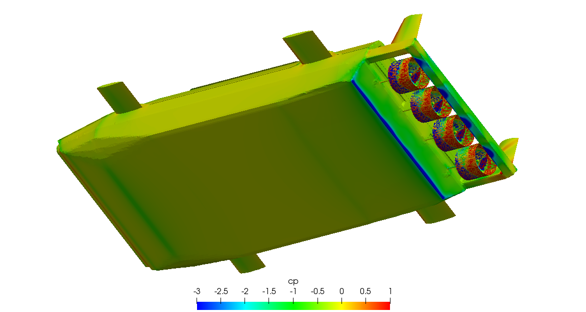
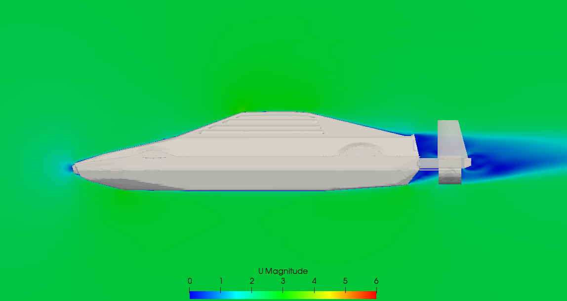
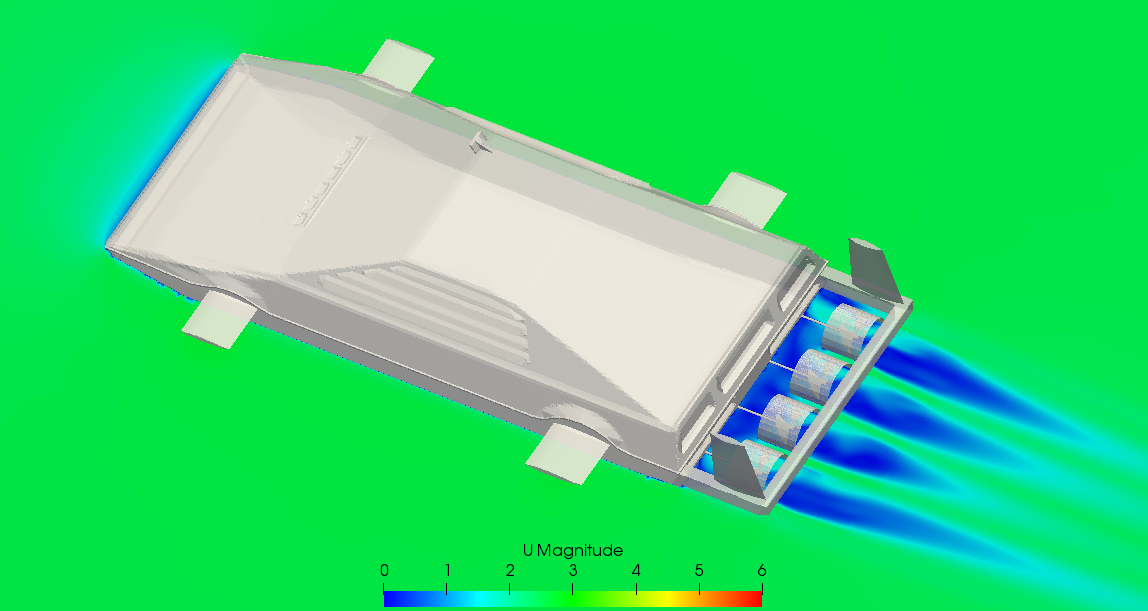
Very interesting things could be analysed on the basis of this model, but for now I will focus only on drag and the effect of the propellers on it.

Drag

Let’s see how they [propellers] alter the drag in the following graph.

Both traces appear identical until the second fin, at which time the influence of the propellers begins to be noticeable. In both cases, the flow of water accelerates behind the vehicle to enter the ducts where the propellers are housed. This causes the pressure to drop, all the more so when the speed of the fluid is higher, causing the drag to increase due to the greater pressure difference between the front and rear of the vehicle.

Moving a little further, we see that once the flow is inside the propellers, the drag variation is different. At low revs the drag increases, while at high revs the drag decreases. This is because in the first case the blades move the water at a lower speed than the submarine, so we would not be pushing.

However, when we increase the rate of rotation, the water is propelled with greater force and the drag becomes negative, which would help us move forward. But then the jet meets the rear crossbeam that breaks it. This crossbeam in the film is not solid, but are two horizontal profiles of a much smaller thickness than what we have represented in our CAD model.

Lift

The same accelerated flow that decreases the base pressure at the rear of the Lotus increasing the drag, increases the pitch moment because the lowest static pressure zone is in the radius where the submarine floor ends.

On the other hand, the chart shows some lift at the height of the propellers. This might seem strange at first because the three blades should cancel each out. Have a look at the image below.

If we look carefully, we can see that when one of the blades pushes the water up, there is a second opposite blade that pushes the water down cancelling the effect of the first blade, and a third that does not push the water vertically. This would be the ideal case —when the flow of water is uniform—, that we can see if we put the slider in the graph below in step-10. But is the upstream flow uniform in our case? By looking at the Y-slices it is evident that this is not the case.

In a very simplified way, in the previous graph we try to show the effect that such non-uniformity could have on the generation of lift by the propellers. And as expected, when the evolution of the blade-generated lift is sinusoidal, the overall result is 0 lift.

Conclusion

In this article we have taken just a brief look at a portion of the results; how the drag and the distribution of pressures on the surface of the submarine vary according to the rotation speed of the propellers. As might be expected, propellers provide thrust from a certain regime on; this increases fluid velocity in the vicinity while reducing static pressure.

Another result, certainly worth mentioning, is the generation of lift in the propeller zone due to the non-uniformity of the flow. It is a finding that certainly deserves a post of it’s own.

References

Oagana, A. (2016). Wet Nellie: The Second Most Famous Bond Car. [online] autoevolution. Available at: https://www.autoevolution.com/news/wet-nellie-the-second-most-famous-bond-car-35087.html [Accessed 23 Mar. 2019].

The Spy Who Loved Me. (1977). [film] Directed by L. Gilbert. UK: Eon Productions.