DrivAer: fastback vs estate back aerodynamics

I own myself a fastback Mazda 6, but also like estate back versions of certain models like the BMW 3-series. So, I’m curious about the aerodynamic performance delivered by both body styles. Luckily enough, the Technical University of Munich has developed a realistic car model intended to replace the Ahmed body used in investigations in automotive aerodynamics. The DrivAer model was introduced circa 2011 and features three body styles: fastback, estate back, and notchback. This styles can be combined with different wheels, underbodies, and engine bay allowing for 18 distinct configurations. The CAD data of the DrivAer model is available on request.

There is also plenty of research carried around those geometries, so that it is possible to validate our simulations.

Computational domain

Although the Master’s thesis by Yazdani (2014) is quite comprehensive, his smallest volume discretization consisted of circa 50 million-cells; well above my personal computational resources, even though I were to consider symmetry. For this reason, I took some hints from the work by Shinde et al. (2013) in order to get a representative enough computational domain with a fraction of the cell-count while keeping drag estimations within 5 % of experimental results.

Mesh

The model simulates a 1:2.5 scaled down DrivAer vehicle inside a virtual wind tunnel of size 28 × 10 × 7 m³. This results in a blockage ratio of 0.57 %. For a symmetry case, we get 9.1 million cells, with 5 boundary layer cells around targeting a y+ of 30.

The mesh was generated with cfMesh. As I was struggling to get a good boundary layer coverage of the DrivAer model using snappyHexMesh —which in turn impaired simulation results—, I turned to this other mesher that claimed to achieve 100 % boundary layer coverage with minimal settings. And I have to admit that I was pleasantly surprised by the results.

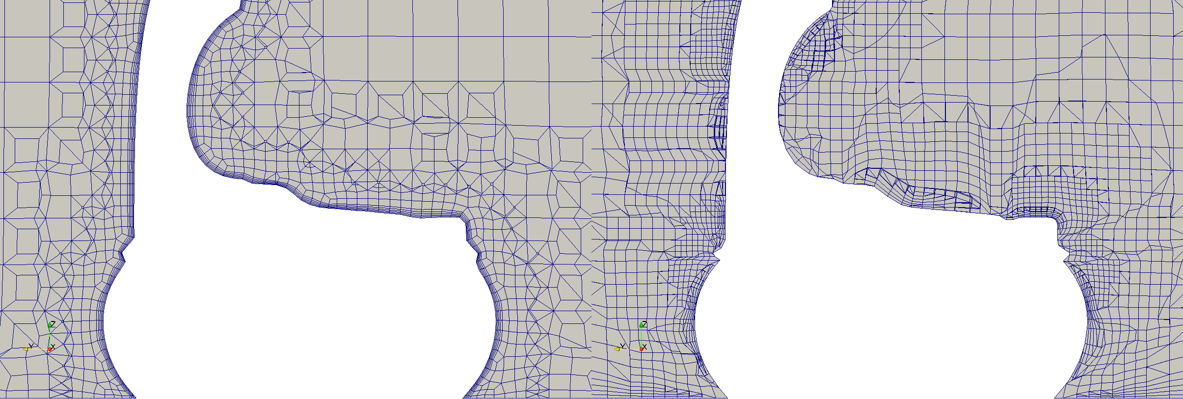
In the image above we can see side by side the results I achieved using both meshers: cfMesh on the left, and snappyHexMesh on the right. The boundary layer coverage I got with snappyHexMesh is chaotic at best —and I tried many different settings and spent a great deal of time at CFD Online looking for settings to improve mesh quality—. With cfMesh, on the contrary, with just a few settings I got a really neat mesh, and in one third of the time.

The only important thing I am not considering for this simulation is MRF; as I don’t know yet how to properly mesh a separate cell zone with cfMesh.

Boundary and initial conditions

Following the settings portrayed by Shinde et al. (2013), the inlet velocity is set to 40 m/s, with turbulent initial conditions estimated following best practice guidelines —turbulent kinetic energy k of 0.0096 m²/s² and specific turbulent dissipation rate ω of 61.935 s^–¹. The following table defines al the boundaries specified at time 0:

Boundary	p	U	k	omega	nut
inlet	zeroGradient	fixedValue uniform (40 0 0)	fixedValue uniform 0.0096	fixedValue uniform 61.935	calculated uniform 0
outlet	fixedValue uniform 0	zeroGradient	zeroGradient	zeroGradient	zeroGradient
tunnel	zeroGradient	slip	kqRWallFunction uniform 0.0096	omegaWallFunction uniform 61.935	nutUSpaldingWallFunction
floor	zeroGradient	movingWallVelocity uniform (40 0 0)	kqRWallFunction uniform 0.0096	omegaWallFunction uniform 61.935	nutUSpaldingWallFunction
car	zeroGradient	movingWallVelocity uniform (0 0 0)	kqRWallFunction uniform 0.0096	omegaWallFunction uniform 61.935	nutUSpaldingWallFunction
symmetry	symmetryPlane	symmetryPlane	symmetryPlane	symmetryPlane	symmetryPlane

Results

The total drag value for the two models corresponds to a configuration with smooth underbody and no rotating wheels. The following table shows the average simulated drag value and the corresponding experimental one from Mack et al (2012) for smooth underbody and stationary ground configuration (GS off).

Model	Expt. Cd	CFD Cd	Error
Fastback	0.249	0.248	-0.40 %	-1 ct
Estate back	0.286	0.273	-4.55 %	-13 ct

Correlation is quite good. Just as is the case with Shinde et al. (2013) and Yazdani (2015), we get better correlation with the fastback model.

The previous plot shows the accumulated drag for both fastback and estate back. We can see the influence of the difference in the geometry of the back as far forward as in the front axis. But in this post I am only going to focus my attention on the rear end where the differences are most noticeable.

Pressure

The most elemental visualisation used to spot drag inducing areas is that of pressure contours —out of the two components of drag, pressure and shear stress, the former plays the leading role—. In the following slideshow we show images of the x-component of the pressure coefficient for both fastback and estateback models.

References

Heft, A. I., Indinger, T., & Adams, N. A. (2012). Experimental and Numerical Investigation of the DrivAer Model (pp. 41-51). ASME.
Hucho, W.-H., & Ahmed, S. R. (1987). Aerodynamics of road vehicles: from fluid mechanics to vehicle engineering. London: Butterworths.
Mack, S., Indinger, T., Adams, N. A., Blume, S., & Unterlechner, P. (2012). The Interior Design of a 40% Scaled DrivAer Body and First Experimental Results (p. 75). ASME.
Shinde, G., Joshi, A., & Nikam, K. (2013). Numerical Investigations of the DrivAer Car Model using Opensource CFD Solver OpenFOAM.
Yazdani, R. (2015). Steady and Unsteady Numerical Analysis of the DrivAer Model (MSc Thesis). Chalmers University of Technology, Göteborg.