Alfa Romeo P2 CFD analysis (pt. 1)
You can’t be a true petrolhead until you’ve owned an Alfa Romeo.
Jeremy Clarkson
And what best Alfa Romeo than an evolution of the first model to win the inaugural Automobile World Championship in 1925 marking the beginning of Alfa Romeo’s legend?

In this Alfa Romeo P2 CFD analysis I will compare drag for different configurations:
- Static and rotating wall boundary condition on the tires. Might try to implement an MRF simulation around to account for the effect of the wheel spokes sometime in the future.
- Without and with driver.
You can have a look at the simulation setup in SimScale.
Contents
Pre-processing
Alfa Romeo P2 geometry and mesh
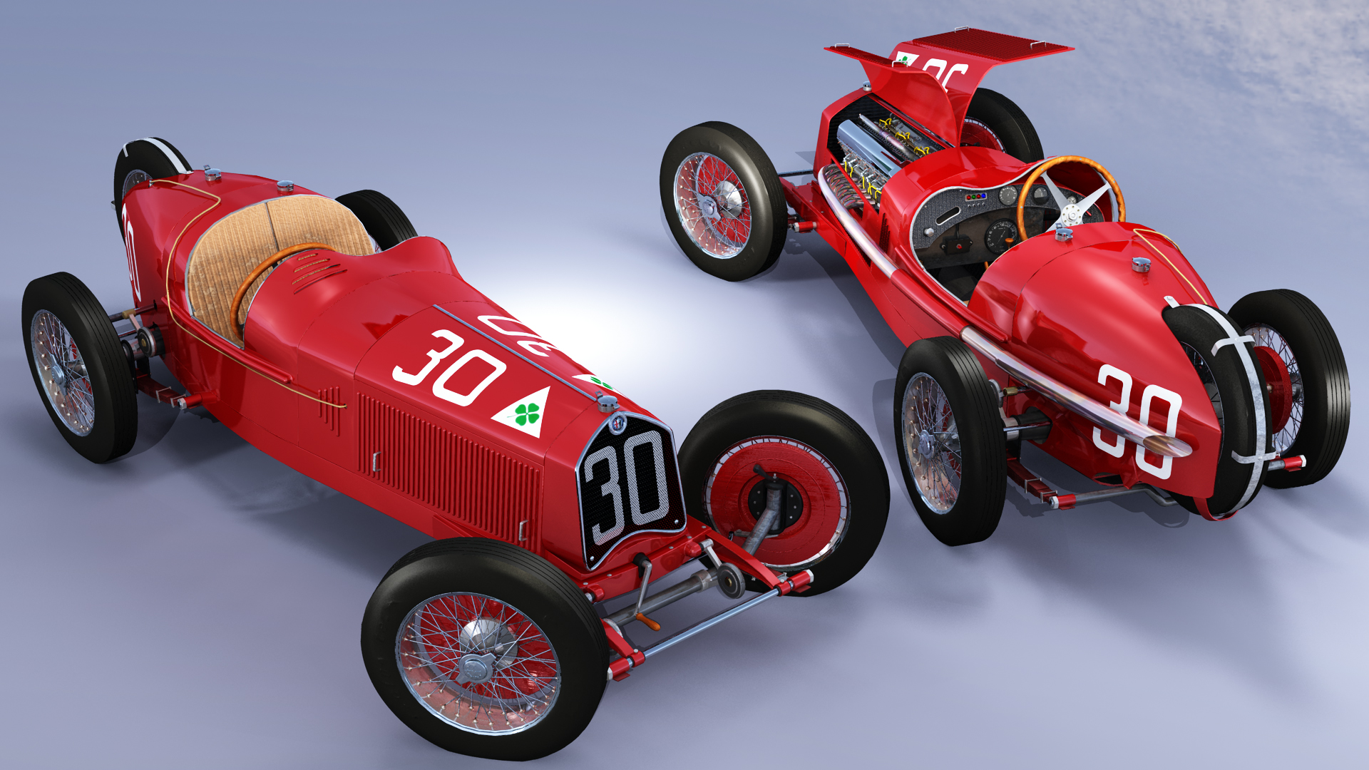
The 3D model of this italian race car is available in GrabCAD. The #30 was driven by Achille Varzi at the 1030 Targa Florio in what would be the P2’s latest victory. The car features a flat radiator, a slot cut down the fuel tank at the rear to host a spare wheel, and the rear springs placed outside the chassis rails.
For the CFD simulations I also wanted to add a driver. For this I took a mannequin from GrabCAD, designed by Emmanuel Mahay. I am analyzing only the one-driver configuration as the 1925 championship regulations prohibited the carrying of riding mechanics, although the cars were still required to have two seats —the 1930 Targa Florio line-up consisted of a driver and assistant mechanic, but this was a non-championship Grand Prix.

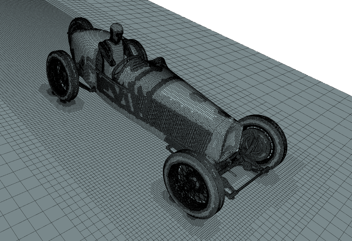
The geometries, both with and without driver, were uploaded to SimScale for discretization. The meshing algorithm is the well-known snappyHexMesh with a base mesh box of dimensions 40 × 10 × 5 m³. That results in a tunnel with a 2.2% blockage ratio. The base cell size is 33 cm, and the smallest cells at a refinement level of 6 are ~5.2 mm side.
The settings yield a rather coarse given the intricacies of the model: ~10.5M cells; 11M cells if we include the driver. This is so in order to contain the size of the model as we are limited to 32 CPUs; not to mention the limitations of my current workstation.

The refinement level is enough to capture the wheel spokes so characteristic of classic cars as can be seen in the picture above. Despite this level of detail, the spokes do not exert their influence in full over the flow; for that, we would have to simulate their rotation with a MRF or a dynamic mesh. In this simulations I just considered the rotation of the tyre by specifying a rotating wall boundary condition.
Boundary and initial conditions
In this simulation I am setting six different boundary conditions:
- Velocity inlet for virtual wind tunnel inlet.
- Pressure outlet for the virtual wind tunnel outlet.
- Moving wall for the virtual wind tunnel floor.
- Slip wall for the rest of the virtual wind tunnel walls.
- No-slip for the vehicle surfaces.
- Rotating wall for the vehicle’s tires.
The velocity is set to 40 m/s (144 km/h) which is slightly below the maximum speed recorder for this race car. This velocity, together with turbulence intensity, eddy viscosity ratio, and kinematic viscosity, is used to calculate the turbulence variables for the k-omega SST turbulence model.
Results
Tire rotation
I ran two simulations with different boundary conditions for the tires. One run with a no-slip wall boundary condition and other run with a rotating wall boundary condition —just for the tire.
The influence of the tire can be seen on the charts below.
It is readily apparent that the blunt front bodywork of this racecar is responsible for nearly half the drag while the streamlined rear-end of the car adds very little. Also, the tire rotation seems to have very little influence on drag. Of course, the wheelspokes would have something different to say on the matter; but for that we would require an alternative approach, e.g., MRF.
If we want to take a closer look at the data, we can plot the delta.
Although small the difference, there is some, specially noticeable in the rear wheel. In the front wheel, there’s a spike in pressure at the back of the wheel, possibly due to the promotion in separation of the upstream-moving face when the tire rotates (Knowles 2005).
Driver
The previous results include no driver. As the Alfa Romeo P2 is an open two-seater, the influence of the driver cannot be neglected. So, I added a mannequin in the place of the driver. These are the results.
| Baseline | Driver | |
| Cd | 0.651 | 0.634 |
| Cd × A | 0.680 | 0.701 |
Here we introduce the concept of drag area. This metric allows us to compare side by side objects of different reference area —by adding the driver we are increasing the frontal area by 0.064 m²—. Just take a look at the drag equation,
$$ D = \frac{1}{2}\rho C_D A v^2$$
If we don’t take into account the differences in frontal area, we might get the wrong impression that by adding a driver we improved the drag of the vehicle, but nothing could be further from the true.
The plot shows that the effect of the driver is appreciable from the start of the cabin interior at 1.5 m as with the driver more pressure builds-up at the firewall which acts on the driving direction.
In following posts I will include some visualizations like cp delta in order to better understand what’s going on. Stay tuned.
References
Knowles, Robin David. 2005. ‘Monoposto Racecar Wheel Aerodynamics: Investigation of Near-Wake Structure & Supporting-Sting Interface.’ PhD Thesis, Cranfield Univesity.
Read more about Alfa’s heritage in these articles by Nicholas Lancaster:
