
SimScale F1 Workshop, a step further
SimScale started, a couple of weeks ago, a series of workshops on F1 aerodynamics in collaboration with Nic Perrinn, creator of the open source LM P1 and Formula 1 cars. You can watch the recording of the first session on Fundamentals of F1 aerodynamics in the following video.
A really interesting workshop to understand a little bit more about the constraints that drive the aerodynamic design of a Formula 1. Concepts such as the Y250 vortex (33:00) and the whole point behind the multiple cascade wing elements and necessity to weaken and burst the outboard vortex (35:20) in order to reduce the drag of the car are briefly explained.
Post-processing is done locally in ParaView, but we have no information on how much drag and downforce the car is generating. Those are aerodynamic forces acting on the body and are due to only two basic sources (Anderson, 2007):
- Pressure distribution over the body surface, and
- Shear stress distribution over the body surface.
The simulations I ran and downloaded have no information of wall shear stress, so we will have to resign ourselves with calculation the forces based only on pressure distribution. Without wall shear stress neither can I generate the Surface LIC visualizations; thus I shall investigate that issue further.
By definition, pressure $p$ acts normal to the surface, and shear stress $\tau$ acts tangential to the surface. The net effect of the $p$ and $\tau$ distributions integrated over the complete body surface is a resultant aerodynamic force $R$ and moment $M$ on the body. We can the split $R$ into components, being the drag $D$ the component of $R$ parallel to $V_\infty$, and the downforce $-L$ the component of $R$ perpendicular to $V_\infty$.
Pressure coeficcient
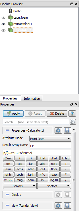
But first, we will compute and visualize the pressure coefficient which is what Nic Perrinn means by rescaling the plot (18:30). The difference, I am going to actually compute the value, which is just
$$ C_p \equiv \frac{p – p_\infty}{\frac{1}{2}\rho_\infty V_\infty^2} \equiv \frac{p – p_\infty}{q_\infty} $$
where $q_\infty$ is the freestream dynamic pressure, and $p_\infty$ is the reference pressure. After we have extracted the block we can use the Filter > Data Analysis > Calculator to simply compute the pressure coefficient. The result is shown in the pictures below.
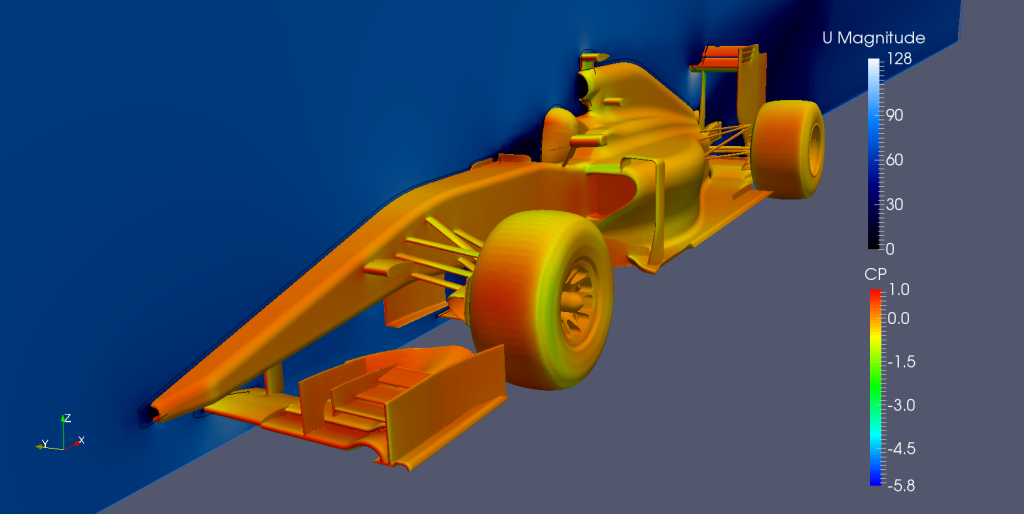
Pressure coefficient over Perrinn’s Open Source Formula 1.
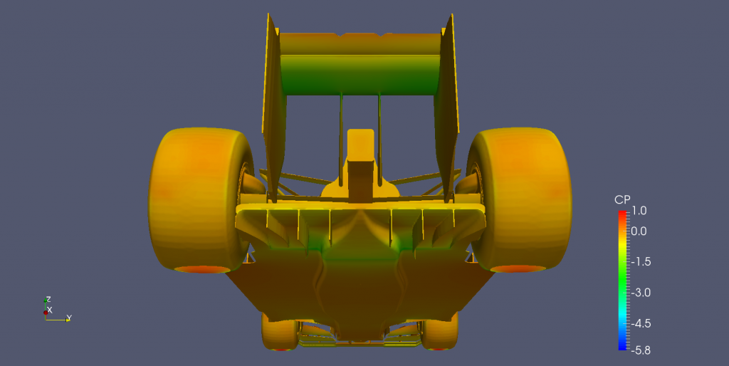
Rear-bottom view of Perrinn’s Open Source F1.
As we can see, the maximum pressure coefficient is 1 while the minimum may extend up to 5.8 times that of the reference dynamic pressure with values around -2 about the suction surface of the rear wing. The suction surface of the rear wing is an area with the higher velocity and lower static pressure; in this case the lower surface. This is the part of the wing which contributes the most to the generation of downforce and should remain as clean as possible. That’s the whole point behind the new wing concept by Koenigsegg as Christian explains.
Drag and downforce coefficients
We can use the same calculator in ParaView to represent the coefficient of drag and downforce. In that case we will want to compute the surface normals first. This generates a new array of vectors called Normals. If we are to calculate the drag coefficient we have to use the following expression: -Normals_X * p / (0.5 * 1.225 * 80^2).
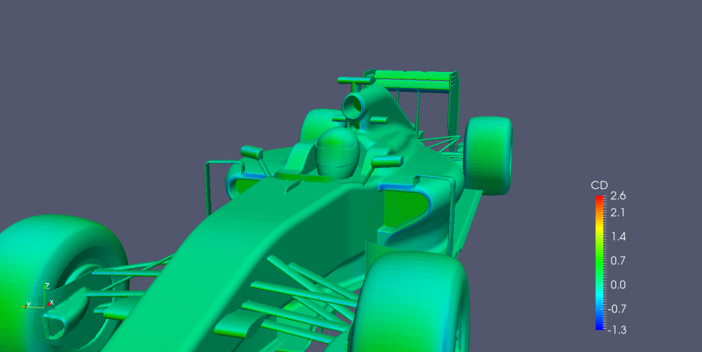
Drag coefficient.
Most of the car is almost neutral in terms of pressure drag; but there are some spots with negative drag. This means that this areas —blue color— are contributing to push the car forward, mainly around the sidepots intake. This is a common effect in jet engine nacelles, but here it is somehow unrealistic as the simulation is not considering the sidepot intakes so that the air that would enter into the car is accelerating around the sidepot.
To obtain the downforce coefficient we have to use the corresponding unit vector component, in this case -Normals_Y.
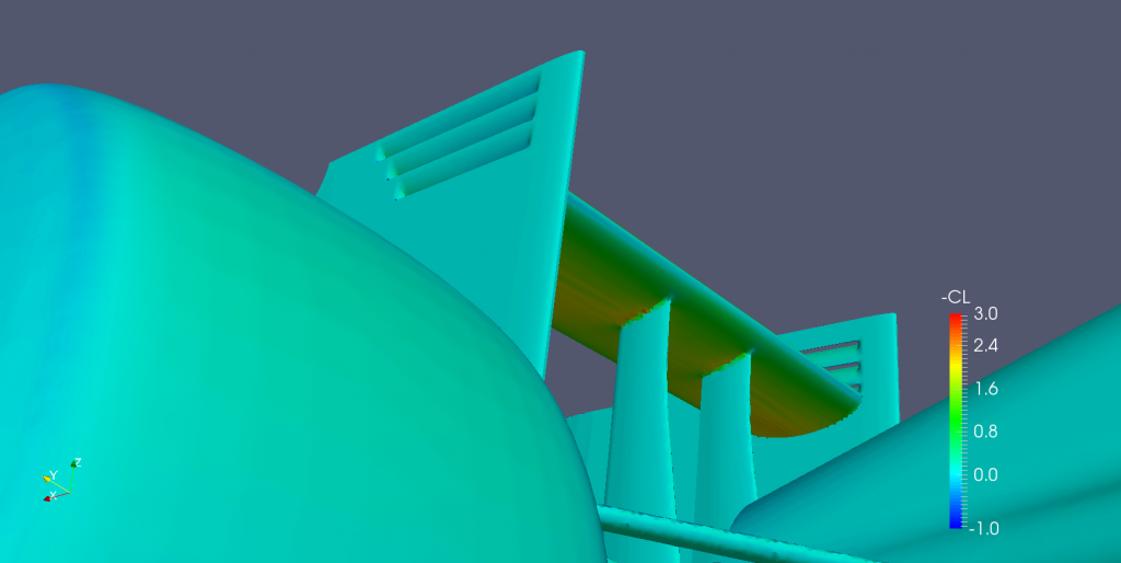
Rear wing downforce coefficient.
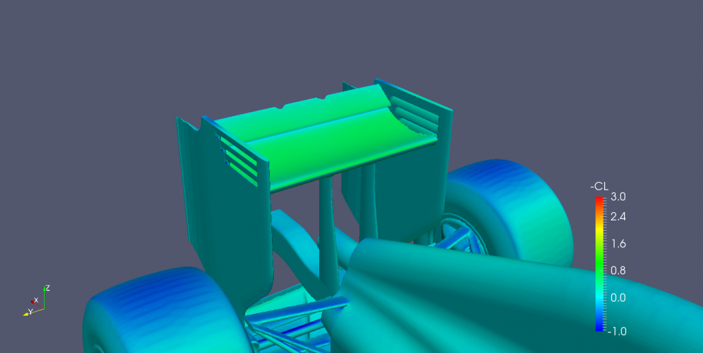
Rear wing downforce coefficient.
The downforce coefficient confirms our early finding; the lower surface is generating about twice the lift compared to the upper surface. The rear wing is also the element that contributes the most to downforce. Next would be the front wing and third the undertray, specially near the diffuser.
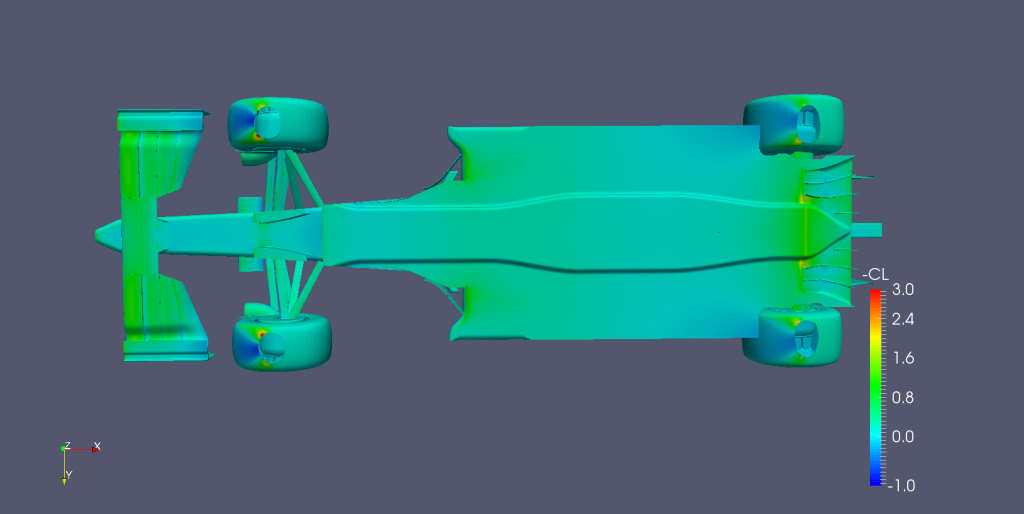
Bottom view downforce coefficient.
The undertray will take advantage of the Bernoulli principle and the relative motion of car and floor —Couette flow— to increase the speed of the air and, as a consequence, the downforce. More on that on a later post.
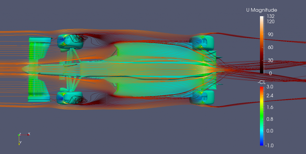
Undertray streamlines.
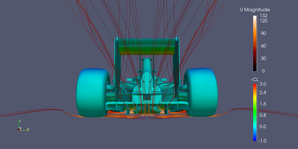
Undertray streamlines exiting through the diffuser.
Remember that you can run your own simulation at SimScale and become the next #F1SimStar.
References
Anderson, J. (2007). Fundamentals of Aerodynamics. 4th ed. New York: McGraw-Hill.