
Physic models in STAR-CCM+ (Part I)
Now that we’ve seen the meshing models available in STAR-CCM+, it is about time to have a look at the physic models solvers used to provide a numerical solution.
In contrast to meshing models where the number of options is limited, the number of choices and combinations within the physic models is almost unbounded. Being that the case, I will break my lecture on physic models into different parts. This is Part I.
Contents
Space
The primary function of the Space models is to provide methods for computing and accessing mesh metrics.
There are four models available in STAR-CCM+, namely
- The Axisymmetric Model
- The Shell Three-Dimensional Model
- The Two-Dimensional Model
- The Three-Dimensional Model
The axisymmetric model
The axisymmetric model is designed to work on two-dimensional axisymmetric meshes. The code solves the case in a 2D domain, but considers the mesh to be swept an angle of 1 radian to give it the third dimension for calculating forces, mass flows, etc. That’s because 2D axisymmetric models represent a slice of the actual 3D model that, if revolved around its axis, would become the original 3D structure. This can lead to reductions of several orders of magnitude for solution time and file size.
The shell three-dimensional model
The shell three-dimensional model is required when modeling heat conduction within a solid shell or modeling fluid films.
The two-dimensional model
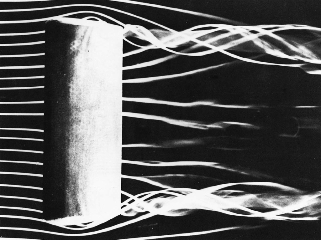
The two-dimensional model is designed to work on two-dimensional meshes. It is comparable to the axisymmetric model in that it represents a 2D slice of a 3D model. This model allows for rapid simulation presuming that variations of conditions in one of the directions are much less important than those in the others —e.g., the CL and CD for a finite wing are not even close to those for the airfoil it’s made of because, in a finite wing, all three spatial directions are relevant due to wing tip effects (see Figure 1). Indeed, airfoil data are frequently denoted as infinite wing data.
The three-dimensional model
The three-dimensional model is designed to work on three-dimensional meshes in cases where all spatial directions are relevant.
Time
Time models in STAR-CCM+ provide solvers that control the iteration and/or unsteady time-stepping. The models available are
- Steady
- Implicit Unsteady
- Explicit Unsteady
- Harmonic Balance
Steady
This model is used for all steady-state calculations; this means that only spatial derivatives are discretized. In steady state calculations we wish to integrate from some arbitrary state to the asymptotic solution in any manner which will get us there in the least amount of computational work.
How do I know in advance whether to perform a steady-state or an unsteady CFD simulation?
I found good guidelines at Symscape.
Implicit unsteady
When considering how to discretize the time derivatives, we need to recognise a major difference between space and time coordinates:
- Most real fluid flow problems are (at least to some extent) elliptic in nature —any forcing introduced has an effect in all directions.
- However, time dependence is purely parabolic —any forcing affects only the future, never the past.
To reflect this, solution methods tend to advance in time in a marching manner, i.e., updating the solution at each time-step.
Considering a generic time-dependent problem
$$ \frac{\partial \phi}{\partial t} = f(t,\phi(t)) $$
integrating with respect to time, over one time step, gives
$$ \phi^{(n+1)} = \phi^{(n)} + \int_t^{t+\Delta t} f(t,\phi(t))\, dt. $$
where the superscript $(n)$ denotes a quantity evaluated at time $t$, and $(n+1)$ at time $t + \Delta t$.
If the integral is approximated using the value of the integrand at the final time, $t + \Delta t$, then we have
$$ \phi^{(n+1)} = \phi^{(n)} f(t+\Delta t, \phi^{(n+1)})\Delta t $$
which is a fully implicit method. This expression cannot be solved in a simple pointwise fashion, since values of $\phi^{(n+1)}$ appear on both the left and right hand sides. In a general case it will thus often require an iterative solution procedure to obtain $\phi^{(n+1)}$.
The following solution was obtained in STAR-CCM+ using an implicit unsteady model.
Explicit unsteady
This model is an alternative to the implicit unsteady model and is only compatible with inviscid and laminar viscous regime models within the coupled energy model.
Approximating the integral on the right hand side using the value of $f$ at the initial time, $t$, then we obtain
$$ \phi^{(n+1)} = \phi^{(n)}+f(t,\phi^{(n)})\Delta t $$
which is a fully explicit method. Once the values at time step $n$ are known, this equation can be applied in a simple explicit fashion to obtain the values of $\phi$ at time step $n + 1$.
The choice between these two approaches is based on the time scales of the phenomena of interest.
Harmonic balance
In STAR-CCM+, the harmonic balance method is a technique for transforming unsteady time-periodic problems into steady-state problems using Fourier series.
The method is inspired on a research paper by Kenneth Hall et al. [6], and allows to solve unsteady flow problems —temporally periodic flows, or even some nearly periodic flows— using steady flow solver techniques. Axial flow turbomachinery, centrifugal machines or helicopter rotors are some of the devices that can benefit from this method.
Motion
Motion is defined as the change in location of a body relative to a particular frame of reference. STAR-CCM+ distinguishes three broad categories:
- Mesh Displacement in Real Time
- Moving Reference Frame in Steady-State
- Harmonic Balance Flutter
Mesh displacement in real time
We include in this category methods that involve actual displacement of mesh vertices in real time and are used for transient analysis.
Moving reference frame in steady-state
A moving reference frame contains the moving part to be solved in steady-state. This approach gives a solution that represents the time-averaged behaviour of the flow, rather tan the time-accurate behaviour.
Harmonic balance flutter
Harmonic balance flutter motion is used in simulations that involve the harmonic balance method with blade vibration.
References
[1] User Guide STAR-CCM+ Version 8.06. 2013.
[2] Van Dyke, M. 1982. An album of fluid motion.
[3] Anderson, J. 2007. Fundamentals of aerodynamics. 4th ed. McGraw-Hill.
[4] Anderson Jr., J. 1995. Computational Fluid Dynamics: The Basics with Applications. 1st ed. McGraw-Hill.
[5] Craft, T.J. 2008. Unsteady Problems.
[6] Hall, K., Thomas, J. and Clark, W. 2002. Computation of Unsteady Nonlinear Flows in Cascades Using a Harmonic Balance Technique. AIAA Journal, 40 (5), pp. 879–886.