Laminar and turbulent steady flow in an S-Bend

I am still having a look at STAR-CCM+’s tutorial, and while I will not post here every single tutorial I follow, I just came across a particular one which happens to be quite similar to one simulation I ran some months ago. So, let’s see if we can compare both solutions despite the differences.

While the simulation I ran in FLUENT was to study the effects of sand erosion in pipe bends, STAR-CCM+ focuses its tutorial in assessing the differences between a laminar and a turbulent flow within a pipe. Nonetheless, pressure and velocity distributions should look alike. Lets take a look.

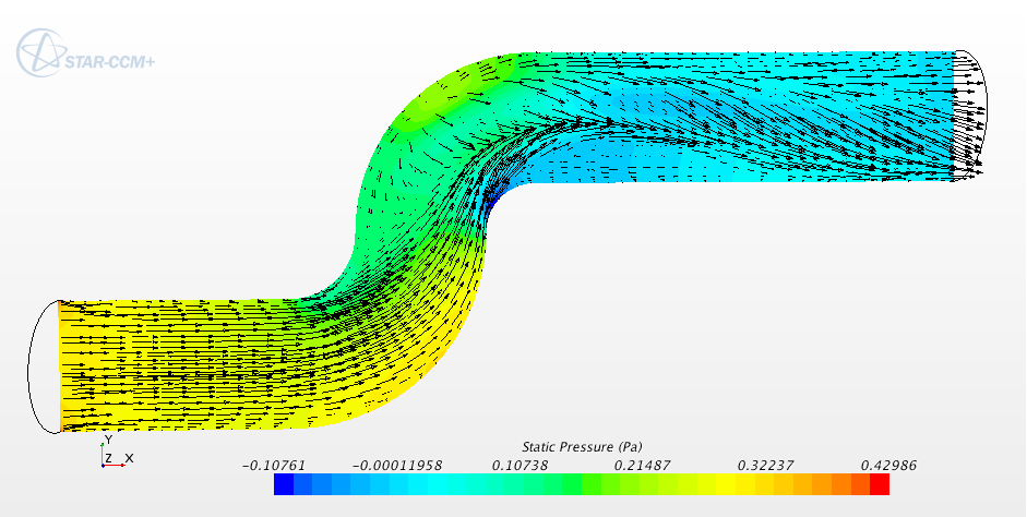
Although geometric dimensions of the pipe are different, the velocity profile —at least along the first segment of the pipe— varies parabolically across the flow. Well, sort of. I guess it is not exactly like the Poiseuille flow because here we impose an inlet flow velocity and the Poiseuille flow is driven uniquely by a pressure gradient. In such a flow, velocity across the flow would be

$$ u = \frac{1}{2\mu} \left( \frac{dp}{dx} \right) (y^2 – Dy) $$

where $\mu$ is the dynamic viscosity, $D$ is the diameter of the pipe, $x$ and $y$ are the Cartesian coordinates and $p$ stands for pressure.

Anyway, the velocity of the slurry analysed with FLUENT of is 10 m/s which makes the flow become turbulent. So, lets take a look at the velocity profile in STAR-CCM+’s turbulent case.

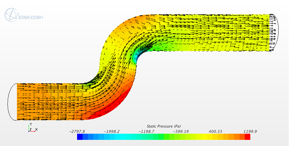
In the turbulent case, the recirculation bubble after the second bend is smaller and the pressure exerted on the wall is greater, more in line with was seen in FLUENT’s simulation.