
Grid sensitivity analysis on the front wing of the McLaren MP4-29 F1 race car
An important aspect to take into account when pushing for a good Computational Fluid Dynamics simulation is the process of verification and validation.
Validation is usually carried out with wind tunnel testing, and that is way out of our scope; unless McLaren engineers were so kind to provide us with the data. Nonetheless, we can do something on the verification side of the process towards a good computational simulation.
Contents
Computational geometry and grid
The computational geometry was generated in Cinema 4D by Juan David Barrera, a 3D and post-production senior composer.
Nuevo Morro Mclaren Modelado… pic.twitter.com/gsIFzJtcyX
— J3DF1 (@erteclas) May 15, 2014
The provided CAD geometry was imported into STAR-CCM+ and a surface wrap was then generated so that the shape could be substracted from a block to get the fluid volume region. Taking advantage of the inherent symmetry of the geometry, only half of the domain is meshed, which drastically reduces the computational requirements.
Three different computational domains were made, with base grid size of 4, 5.66 and 8 cm (ratio r = 1.41). The computational domains have dimensions $L\times X\times H = 20\times 5 \times 5 \text{ m}^3$. The blockage ratio is 0.6 %. The total number of cells is 496654, 892642 and 1767964. A detailed view of the intermediate grid is given in Fig. 1.
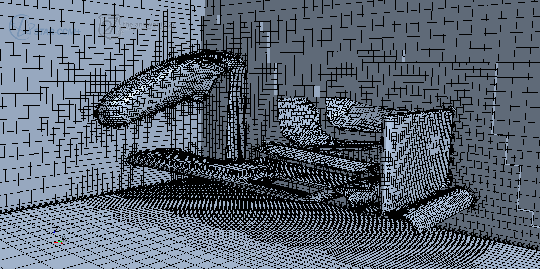
Figure 1. Mesh for the intermediate grid with ~0.9M cells.
Boundary conditions and solver settings
At the inlet of the domain, a constant wind field profile is imposed, the reference wind speed being 50 kph (~13.89 m/s). The floor is of type wall with tangential velocity matching that of the inlet air velocity.
Closure of the RANS equations is obtained with the realizable k–ε turbulence model with two-layer all y+ wall treatment.
Convergence was assessed by monitoring drag and downforce generated by wing, winglets and nose. Less than 1000 iterations were needed to reach a satisfactory solution.
Richardson extrapolation
If the grid refinement is performed with constant r, the order of the scheme p and the discretization error ε can be estimated by
$$ p \approx \frac{\log \left( \frac{ f_3 – f_2}{f_2 – f_1} \right) }{\log r} \qquad \varepsilon = \frac{f_1 – f_2}{r^p – 1} $$
where f is the solution, subscript 1 indicating the fines grid. An estimate of the exact solution is then given by
$$F = f_1 + \varepsilon$$
A rough estimation of the independent grid solution is given below
The difference between the middle grid and the fine grid is 0.6 % (drag) and 1.5 % (downforce). The difference between the fine grid and the estimated grid independent solution is 1.0 % for both drag and downforce. On the other hand, the middle grid is off by 1.6 % and 2.5 %, respectively.
Further analysis
A middle grid with mesh refinement on high gradient zones will be used for further analysis. This way, we can approximate the solution to that of the fine mesh without dramatically increasing the computational cost.
Acknowledgements
This study was performed in STAR-CCM+ 9.02 using a PoD license, thanks to CD-adapco’s Global Academic Program. Special thanks to Juan David Barrera who kindly provided the CAD geometry for analysis.
References
[1] Larsson, T., Sato, T. and Ullbr, (2005). Supercomputing in F1–Unlocking the Power of CFD.
[2] Roache, P. (1997). Quantification of uncertainty in computational fluid dynamics. Annual Review of Fluid Mechanics, 29(1), pp.123–160.
[3] Tu, J., Yeoh, G. and Liu, C. (2013). Computational fluid dynamics: A practical approach. 2nd ed. Waltham, Mass.: Butterworth-Heinemann.