
Dyson’s Air Multiplier with STAR-CCM+
As I mentioned in a previous post, I was curious about how Dyson’s Air Multiplier worked. There is a quite interesting video in YouTube where Sir James Dyson explains how it works:
But I wanted to go a step further and simulate the pathlines all by myself, just as we can see in this other video:
Contents
Geometry
To reproduce the geometry as closely as possible I took some measurements from Gammack et al. [1]. Although the drawings depicted in the Patent are just a first approximation to the final contour of the profile used in the actual fans, it can be used to get some preliminary results. Later on, by using Adjoint solvers, this geometry can be optimized based on a cost function of our choosing.
Having defined the blade shape in CATIA, the mesh generated is shown in Figure 1. The mesh is generated in 2D, as I will use the axisymmetric model to simulate the fluid flow.

Figure 1. Automatic trimmed mesh for the Dyson replica fan blade.
Physics models and boundary conditions
Once we have the geometry defined it’s time to define the physics models to be used and the boundary conditions applied to each surface.
According to Geere [2], the Reynolds at the nozzle is as low as 1615, for which the flow can be assumed as laminar. Furthermore, top speed around the blade is approximately 24.5 m/s (~0.07 Mach), thus we can accept incompressible flow for which we can use the segregated flow models.
We know that the dynamic pressure is

and that, according to Bernoulli’s principle in its simplified form, we can state that

where p0 is the total pressure. So, if we define the inlet as an stagnation inlet, the total pressure we need to stablish to get the desired speed of 24.5 m/s is of 246.85 Pa above our reference pressure.
The rest of the boundary conditions are defined as axis, wall and free stream in accordance with what each one of the boundaries represents.
Preliminary results
In Figure 2 we can see the velocity contours generated by the fan. As we can see, a top speed of 22.3 m/s is achieved in the nozzle, which is very close to the desired value of 24.5 m/s. Also, in Figure 3 we can see how the air exiting the nozzle drags the surrounding air particles to generate a gentle breeze of about 3 m/s along the axis of the fan.
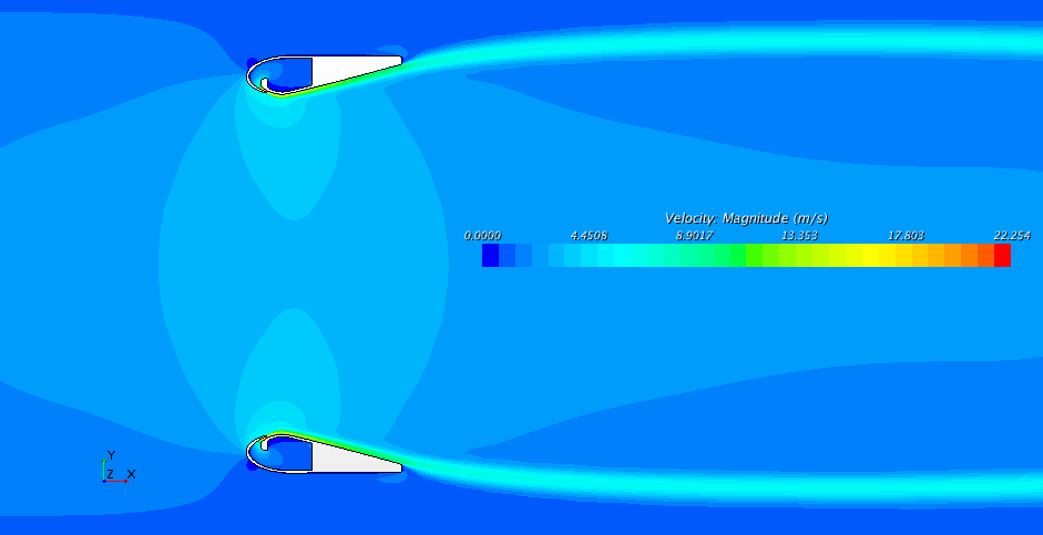
Figure 2. Contours of velocity.
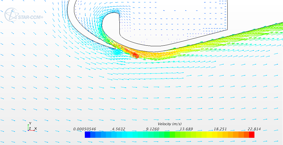
Figure 3. Velocity vectors near the nozzle.
Further analysis can be done along with mesh refinement around critical areas and proper physic models selection.
Enjoy.
References
[1] Gammack, P.D., Nicolas, F. and Simmonds, K.J. 2012. Fan. US Patent 8308445.
[2] Geere, D. 2009. How Dyson’s Air Multiplier works. [online] Available at: http://www.pocket-lint.com/news/98959-how-dysons-air-multiplier-works [Accessed: 26 Jun 2013].